Review of connection between z-score, p-value, and chi2 stat

Review connection between Zscore, p-value, Chi2 statistics

Notice that the estimated effect size divided by the standard error behaves like a normal(0,1) random variable when the sample size is large enough:

\[ Z = \frac{\hat\beta}{\text{se}(\hat\beta)}\] \[Z \approx N(0,1) ~~~~~~ \text{as } n \rightarrow \infty\] Let’s simulate zscore vector under the null hypothesis.

nsim = 5000
set.seed(2021021001)
zvec = rnorm(5000, mean=0, sd=1)

Calculate the p-value (probability that a normal r.v. will be as large or larger in magnitude than the |zscore|

pvec = pnorm(-abs(zvec)) * 2 ## two-tailed
## check pvec is uniformly distributed
hist(pvec,main="is this uniformly distributed?")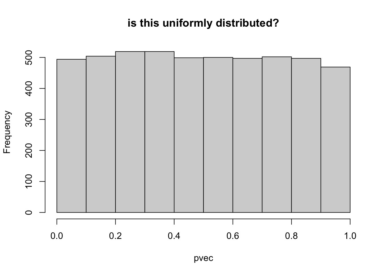

## remember that if square the a normal r.v. you get chi2 r.v. with one degree of freedom
z2vec = zvec^2
## compare with chi2 rv. with 1 degree of freedom by simulating chi2,1 and qqplot
chi2vec = rchisq(nsim,df=1)
qqplot(chi2vec,z2vec,main="compare of zscore^2 and a chi2 r.v."); abline(0,1)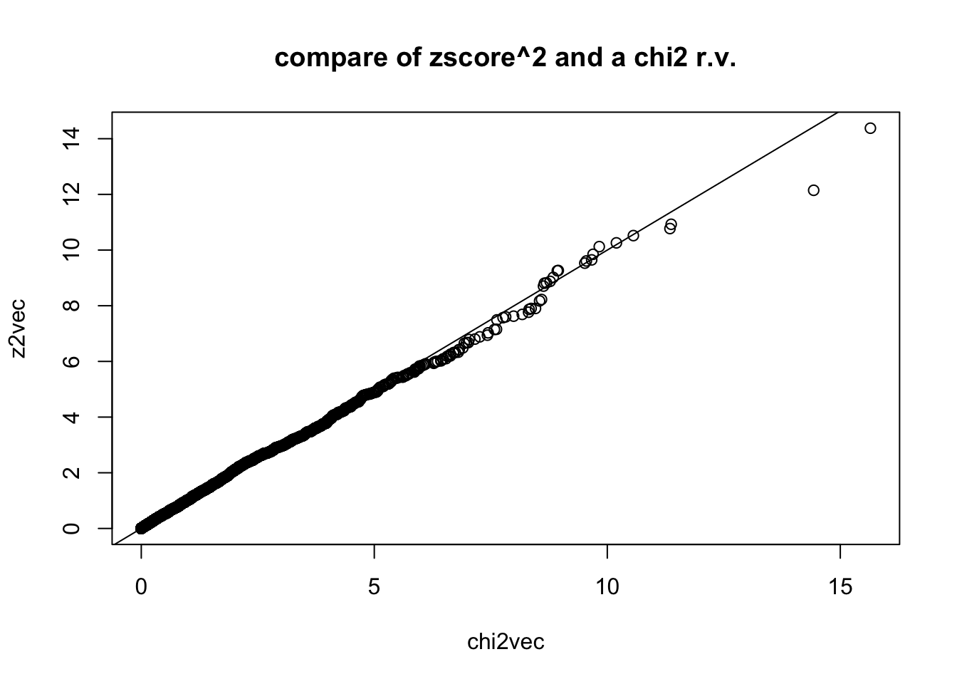

## test whether the distributions of z2vec and chi2vec are different using the Kologorov Smirnov test
ks.test(z2vec,chi2vec)

## 
##  Two-sample Kolmogorov-Smirnov test
## 
## data:  z2vec and chi2vec
## D = 0.019, p-value = 0.3275
## alternative hypothesis: two-sided

## for reference, let's compare two chi2,1 r.v.'s qqplot
chi2vec_2 = rchisq(nsim,df=1)
qqplot(chi2vec,chi2vec_2,main="qqplot of two chi2,1 r.v."); abline(0,1)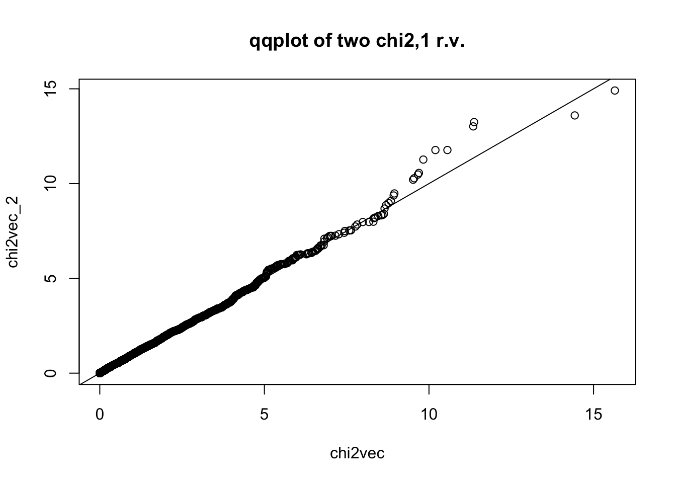

ks.test(chi2vec,chi2vec_2)

## 
##  Two-sample Kolmogorov-Smirnov test
## 
## data:  chi2vec and chi2vec_2
## D = 0.0158, p-value = 0.5605
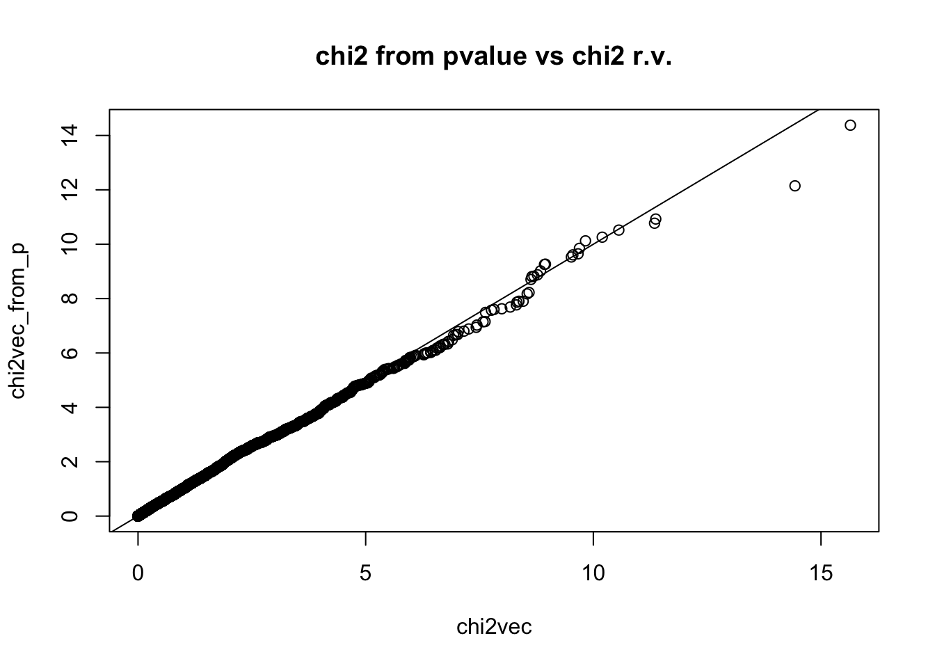
## alternative hypothesis: two-sided

Sometimes you get the p-value instead of the zscore, you can generate chi2 by inverting the relationship.

chi2vec_from_p = qnorm(pvec / 2)^2
qqplot(chi2vec,chi2vec_from_p,main="chi2 from pvalue vs chi2 r.v."); abline(0,1)