Lecture 1: introductions and brief review of probability & statistics

Haky Im

2022-01-10

Categories: Lecture

Brief description of the course

Variation in our genes determine in part variation in phenotypes such as height, BMI, predisposition to diseases, etc. In this course, we are going to learn concepts and techniques to map genes to phenotypes and their underlying mechanisms.
We will focus on complex traits and diseases for which a combination of genetic and environmental factors determine the outcome.

Logistics

The 2022 syllabus has all the relevant information.

Round of introduction (~1’ per person)

We’ll do a round of introductions. Each person will tell us the following

Name, preferred name
Why did you sign up for the course
tell us something either very interesting or very boring about yourself, no need to clarify which one you chose

Learning objectives

Review of concepts in probabiliy and statistics

Bayes Rule
Random variables and probability distributions
Maximum likelihood principle (ML)
Parameter estimation with ML
Bayesian statistics

Lecture notes and other useful material

Review probability
Maximum Likelihood Estimation
Bayesian Inference
Probability cheatsheet: this cheatsheet will be handy throughout the course for your reference. It’s a highly condensed summary of this excellent book by Blitzstein & Hwang, freely available here.

Review

Today, we will review some concepts in probability, establish a common terminology, and go over basic examples in statistical inference using maximum likelihood estimations and Bayesian inference.

Probability

You may want to check the Review notes for a summary of definitions and some hints for you.

Conditional Probability. What is the definition of conditional probabiliy of an event A given event B?
Write \(P(A|B)\) as a function of \(P(A \cap B)\) and \(P(B)\)
Bayes Rule

\[P(A|B) = \frac{P(B|A)\cdot P(A)}{P(B)}\]

Derive the Bayes Rule using the definition of conditional probability
Law of Total Probability: this law can be used to simplify the calculation of the probability of an event B.
Random Varibles: Are real-valued functions of some random process. For example, the number of tails when tossing a fair coint 10 times. The height in cm of a student selected randomly from the Uchicago 2024 class.
is the set {head, tail, tail} a random variable?
is a function that takes value 1 when a coin lands head and 0 otherwise a random variable?
Independence of Random Variables
Expectation, Variance, Covariance of Random Variables
Examples of common distributions
- Bernoulli
- Binomial
- Normal/Gaussian
Indicator function random variable

Maximum likelihood estimation (MLE)

Maximum likelihood estimation is one of the fundamental tools for statistical inference. Basically, we select the parameter value that maximizes the likelihood.

Let’s start by defining the likelihood. It’s a function of the data and the parameters of our model.

\[\text{Likelihood} = P(\text{data}|\theta)\]

Example: coin toss

We toss a coin that has an unknown probability \(\theta\) of landing on head. We tossed the coin once and get H.

data: the coin lands on head
parameter \(\theta\)
likelihood = \(P(\text{data}|\theta)\) = \(\theta\)

Example: two independent coin tosses

data: the coins land (H,T)
parameter \(\theta\)
likelihood = \(P(\text{data}|\theta)\) = \(\theta \cdot (1-\theta)\)

Example: ten independent coin tosses

data: the coins land (H,H,T,H,T,H,H,H,H,H)
parameter \(\theta\)
likelihood = \(P(\text{data}|\theta)\) = \(\theta \cdot \theta \cdot (1-\theta) \cdot \theta \cdot (1-\theta) \cdot \theta \cdot \theta \cdot \theta \cdot \theta \cdot\theta\) = \(\theta^8 \cdot (1-\theta)^2\)

Let’s plot this likelihood as a function of \(\theta\)

n = 10
y = 8
likefun = function(theta) {theta^y * (1 - theta)^(n-y)} 
curve(likefun,from = 0,to = 1, main=paste("n = ",n,";  y = ",y),
xlab="theta", ylab="likelihood")
abline(v=y/n,col='gray')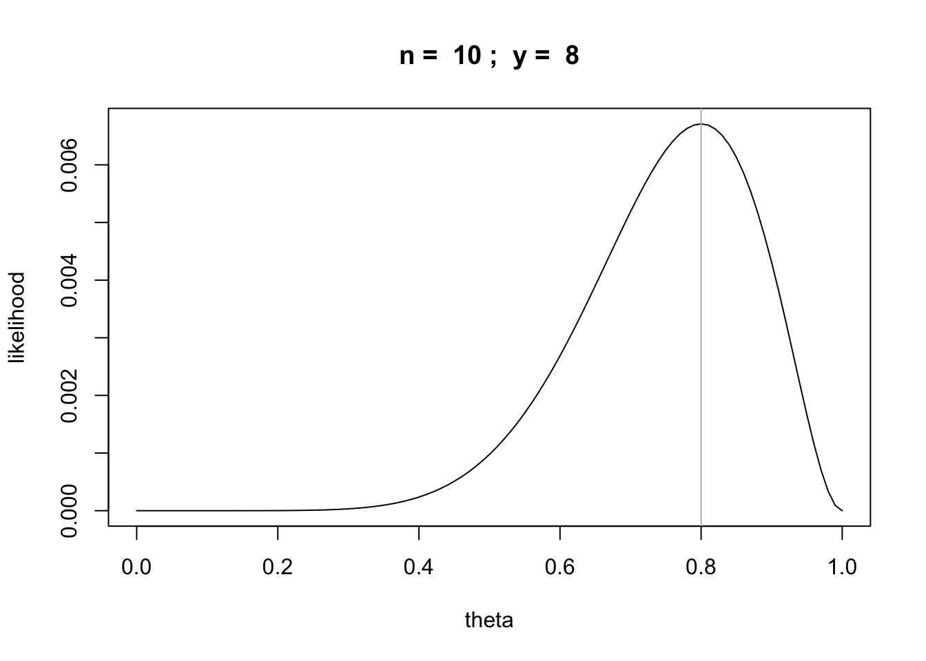

What if we doubled the number of tosses and got 16 heads?

n = 20
y = 16
likefun = function(theta) {theta^y * (1 - theta)^(n-y)} 
curve(likefun,from = 0,to = 1, main=paste("n = ",n,";  y = ",y),
xlab="theta", ylab="likelihood")
abline(v=y/n,col='gray')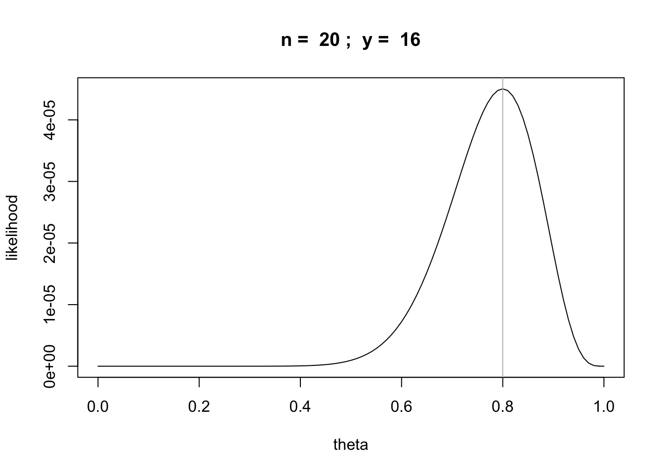

Question: How would you calculate the MLE as a function of the number of tosses in general?

Question: What if we got 10 heads in ten tosses? Can we use the same strategy?

n = 10
y = 10
likefun = function(theta) {theta^y * (1 - theta)^(n-y)}
curve(likefun,from = 0,to = 1, main=paste("n = ",n,";  y = ",y),xlab="theta", ylab="likelihood")
abline(v=y/n,col='gray')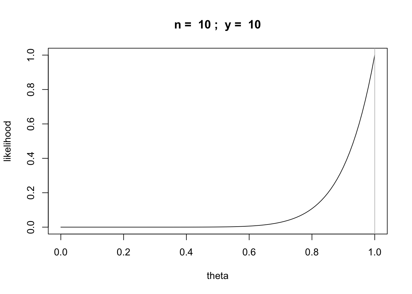

Question: How does the number of tosses change the likelihood function?

Example: normally distributed random variables

data: \(x_1= 0.2\) and \(x_2=-2\)
parameter \(\mu\), \(\sigma^2\)
likelihood = \(f(0.2; \mu, \sigma^2) \cdot f(-2; \mu, \sigma^2)\)

Recall that the probability density function for a normally distributed random variable is

\[f(x; \mu, \sigma^2) = \frac{1}{\sqrt{2 \pi \sigma^2}} \exp[-(x-\mu)^2/(2\sigma^2)]\]

Write down the likelihood for this data

Bayesian Inference

The goal is to learn the parameter \(\theta\) given the data by calculating the posterior distribution

\[P(\theta | \text{data})\] Question: how is this different from the likelihood?

How does this relate to the likelihood?

\[P(\theta | \text{data}) = P(\text{data} | \theta) \cdot P(\theta) / P(\text{data})\] But the normalizing factor \(P(\text{data})\) can be difficult to calculate so we try to extract as much information as possible from the unnormalized posterior

\[P(\theta | \text{data}) \propto P(\text{data} | \theta) \cdot P(\theta)\]

Example: binomial random variable

Let \(y\) be the number of successes in \(n\) trials of some experiment.

unnorm_posterior = function(theta) {theta^y * (1 - theta)^(n-y)}

n = 10
y = rbinom(1,n,0.6)
curve(unnorm_posterior,from = 0,to = 1, main=paste("n = ",n,";  y = ",y))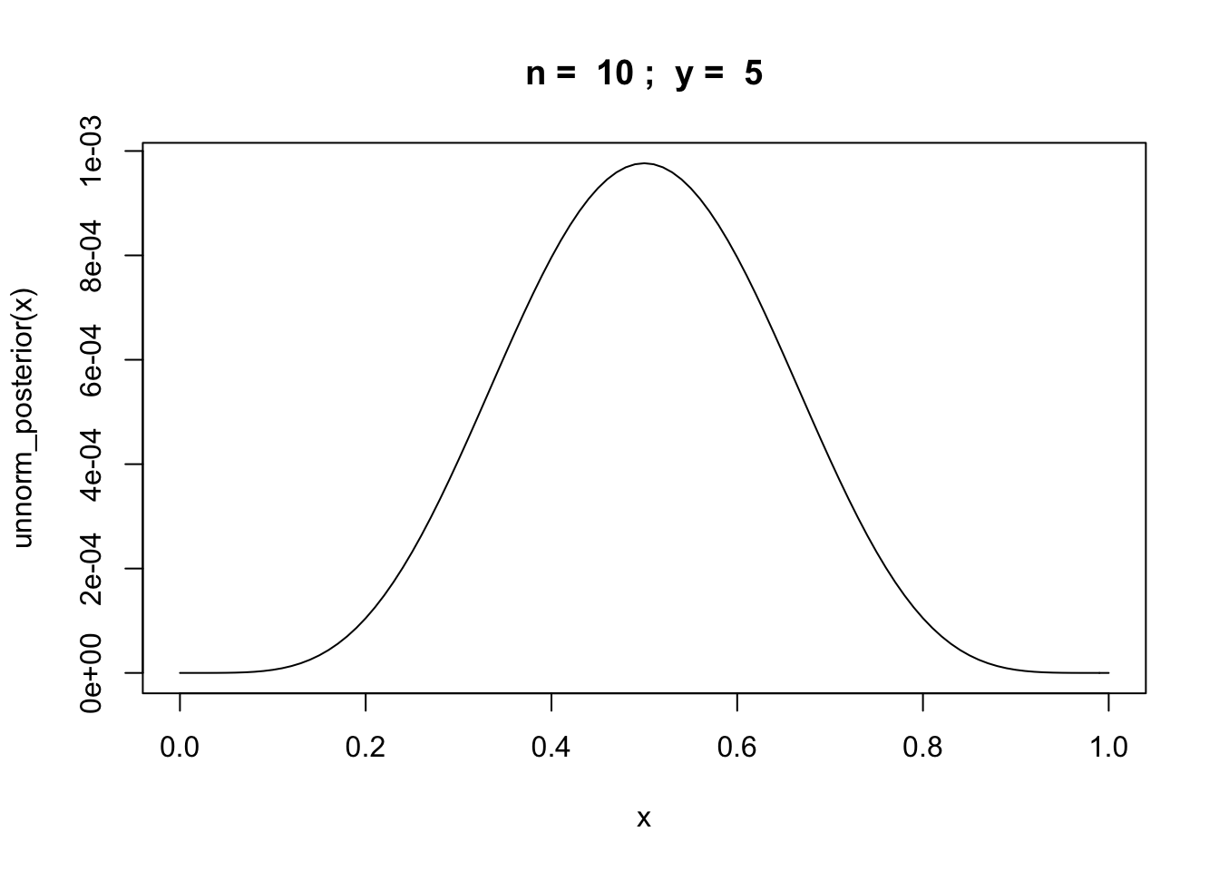

n = 100
y = rbinom(1,n,0.6)
curve(unnorm_posterior,from = 0,to = 1, main=paste("n = ",n,";  y = ",y))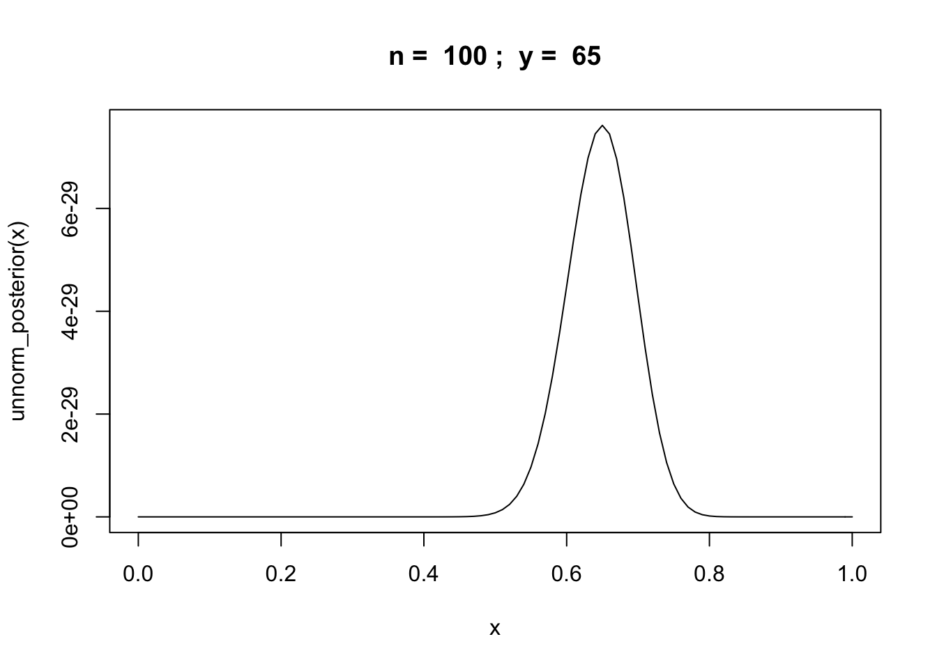

n = 1000
y = rbinom(1,n,0.6)
curve(unnorm_posterior,from = 0,to = 1, main=paste("n = ",n,";  y = ",y))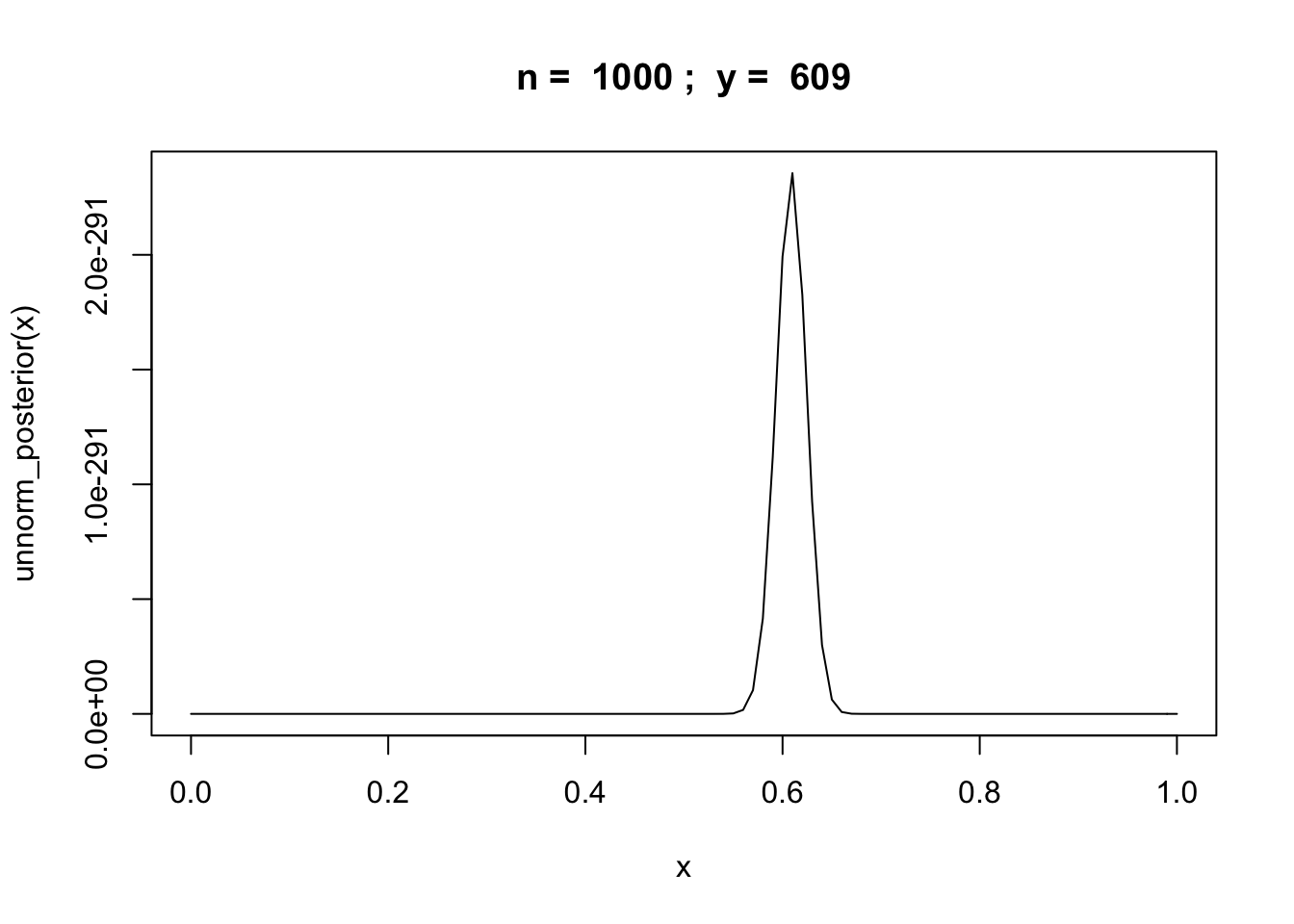

Homework problems

Other problems will be distributed during lab sessions.

References

Blitzstein, Joseph K et al. Introduction to Probability, Second Edition (Chapman & Hall/CRC Texts in Statistical Science) (p. 63). CRC Press. available free online here
Gelman, Andrew et al. Bayesian Data Analysis (Chapman & Hall/CRC Texts in Statistical Science) CRC Press.

Claussnitzer, Melina, Judy H Cho, Rory Collins, Nancy J Cox, Emmanouil T Dermitzakis, Matthew E Hurles, Sekar Kathiresan, et al. 2020. “A Brief History of Human Disease Genetics.” Nature 577 (7789): 179–89.