Lecture 6 - Population Structure

Haky Im

2021-01-31

Categories: Lecture

Learning Objectives

Define population structure
Go through examples of manifestation of population strucutre
Learn methods to correct for population structure
- genomic control
- principal component analysis

Material for the class

Download notes on population structure from here

Prerequisites for running the analysis below

plink installed in ~/bin/
Rstudio is installed
tidyverse package installed
devtools package installed

download data from here TODO box link here

if(!file.exists(glue::glue("~/Downloads/analysis_population_structure.tgz")))
{
  system(glue::glue("wget -O ~/Downloads/analysis_population_structure.tgz https://uchicago.box.com/shared/static/zv1jyevq01mt130ishx25sgb1agdu8lj.tgz"))
  ## tar -xf file_name.tar.gz --directory /target/directory
  system(glue::glue("tar xvf ~/Downloads/analysis_population_structure.tgz --directory ~/Downloads/")) 
}
work.dir ="~/Downloads/analysis_population_structure/"
system(glue::glue("tree {work.dir}"))

library(tidyverse)
## load qqunif function
devtools::source_gist("38431b74c6c0bf90c12f")

Test Hardy Weinberg equilibrium with population structure

What’s the population composition?

popinfo = read_tsv(paste0(work.dir,"relationships_w_pops_051208.txt"))

## 
## ── Column specification ────────────────────────────────────────────────────────
## cols(
##   FID = col_character(),
##   IID = col_character(),
##   dad = col_character(),
##   mom = col_character(),
##   sex = col_double(),
##   pheno = col_double(),
##   population = col_character()
## )

popinfo %>% count(population)

## # A tibble: 11 x 2
##    population     n
##  * <chr>      <int>
##  1 ASW           90
##  2 CEU          180
##  3 CHB           90
##  4 CHD          100
##  5 GIH          100
##  6 JPT           91
##  7 LWK          100
##  8 MEX           90
##  9 MKK          180
## 10 TSI          100
## 11 YRI          180

samdata = read_tsv(paste0(work.dir,"phase3_corrected.psam"),guess_max = 2500)

## 
## ── Column specification ────────────────────────────────────────────────────────
## cols(
##   `#IID` = col_character(),
##   PAT = col_character(),
##   MAT = col_character(),
##   SEX = col_double(),
##   SuperPop = col_character(),
##   Population = col_character()
## )

superpop = samdata %>% select(SuperPop,Population) %>% unique()
superpop = rbind(superpop, data.frame(SuperPop=c("EAS","HIS","AFR"),Population=c("CHD","MEX","MKK")))

Effect of population structure in Hardy Weinberg equilibrium

## what happens if we calculate HWE with this mixed population?
if(!file.exists(glue::glue("{work.dir}output/allhwe.hwe")))
system(glue::glue("~/bin/plink --bfile {work.dir}hapmapch22 --hardy --out {work.dir}output/allhwe"))
allhwe = read.table(glue::glue("{work.dir}output/allhwe.hwe"),header=TRUE,as.is=TRUE)
hist(allhwe$P)

qqunif(allhwe$P,main='HWE HapMap3 All Pop')

## Warning in qqunif(allhwe$P, main = "HWE HapMap3 All Pop"): thresholding p to
## 1e-30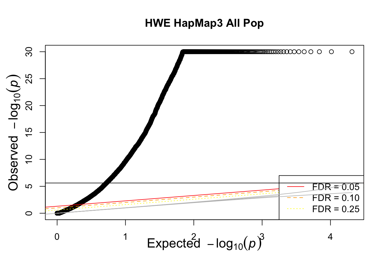

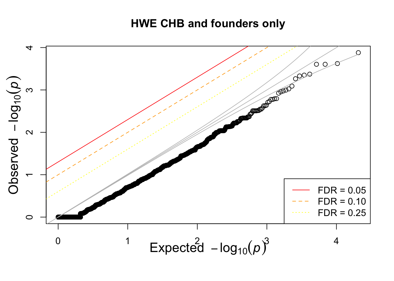
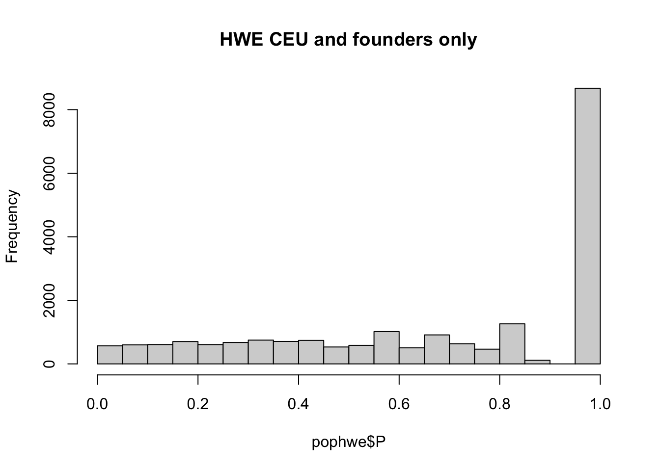
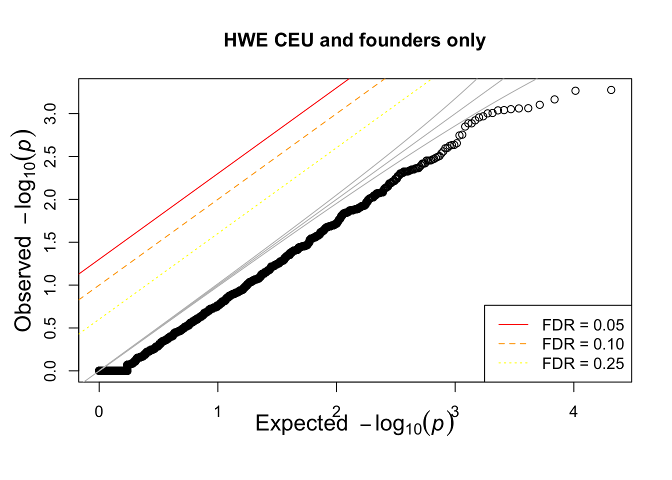
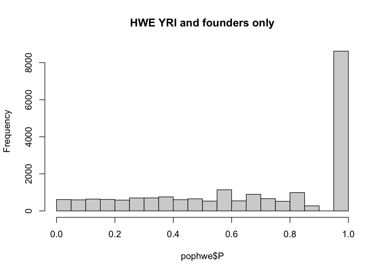
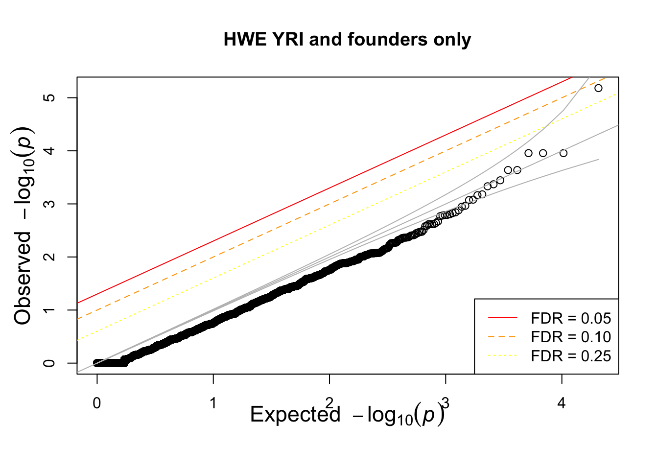
What if we calculate with single population?

pop = "CHB"
pop = "CEU"
pop = "YRI"
for(pop in c("CHB","CEU","YRI"))
{
  ## what if we calculate with single population?
  popinfo %>% filter(population==pop) %>%
    write_tsv(path=glue::glue("{work.dir}{pop}.fam") )
  if(!file.exists(glue::glue("{work.dir}output/hwe-{pop}.hwe")))
  system(glue::glue("~/bin/plink --bfile {work.dir}hapmapch22 --hardy --keep {work.dir}{pop}.fam --out {work.dir}output/hwe-{pop}"))
  pophwe = read.table(glue::glue("{work.dir}output/hwe-{pop}.hwe"),header=TRUE,as.is=TRUE)
  hist(pophwe$P,main=glue::glue("HWE {pop} and founders only"))
  qqunif(pophwe$P,main=glue::glue("HWE {pop} and founders only"))
}

## Warning: The `path` argument of `write_tsv()` is deprecated as of readr 1.4.0.
## Please use the `file` argument instead.
## This warning is displayed once every 8 hours.
## Call `lifecycle::last_warnings()` to see where this warning was generated.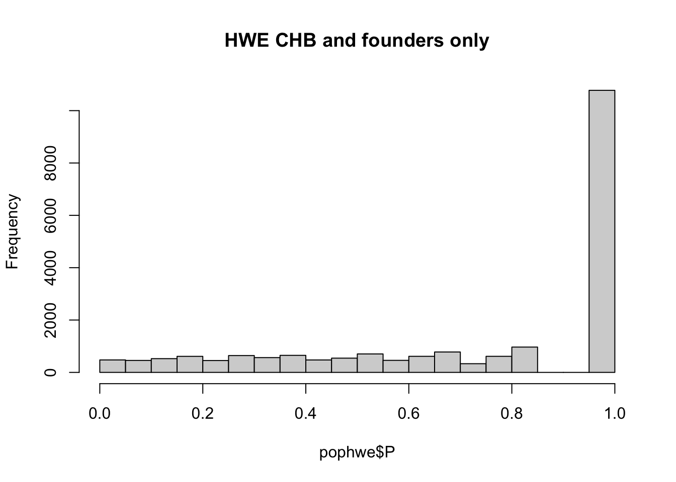

Effect of population stratification on GWAS

GWAS on a growth phenotype in HapMap samples

## read igrowth
igrowth = read_tsv("https://raw.githubusercontent.com/hakyimlab/igrowth/master/rawgrowth.txt")

## 
## ── Column specification ────────────────────────────────────────────────────────
## cols(
##   IID = col_character(),
##   sex = col_double(),
##   pop = col_character(),
##   experim = col_double(),
##   meas.by = col_double(),
##   serum = col_character(),
##   growth = col_double()
## )

## add FID to igrowth file
igrowth = popinfo %>% select(-pheno) %>% inner_join(igrowth %>% select(IID,growth), by=c("IID"="IID"))
write_tsv(igrowth,path=glue::glue("{work.dir}igrowth.pheno"))
igrowth %>% ggplot(aes(population,growth)) + geom_violin(aes(fill=population)) + geom_boxplot(width=0.2,col='black',fill='gray',alpha=.8) + theme_bw(base_size = 15)

## Warning: Removed 130 rows containing non-finite values (stat_ydensity).

## Warning: Removed 130 rows containing non-finite values (stat_boxplot).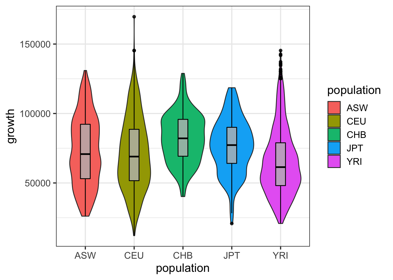

summary( lm(growth~population,data=igrowth) )

## 
## Call:
## lm(formula = growth ~ population, data = igrowth)
## 
## Residuals:
##    Min     1Q Median     3Q    Max 
## -58821 -18093  -2242  15896  98760 
## 
## Coefficients:
##               Estimate Std. Error t value Pr(>|t|)    
## (Intercept)    73080.8      938.2  77.894  < 2e-16 ***
## populationCEU  -2190.1     1175.4  -1.863   0.0625 .  
## populationCHB   9053.1     2043.9   4.429 9.73e-06 ***
## populationJPT   3476.8     2034.8   1.709   0.0876 .  
## populationYRI  -7985.2     1137.2  -7.022 2.61e-12 ***
## ---
## Signif. codes:  0 '***' 0.001 '**' 0.01 '*' 0.05 '.' 0.1 ' ' 1
## 
## Residual standard error: 24160 on 3591 degrees of freedom
##   (130 observations deleted due to missingness)
## Multiple R-squared:  0.0345, Adjusted R-squared:  0.03342 
## F-statistic: 32.08 on 4 and 3591 DF,  p-value: < 2.2e-16

## run plink linear regression only if it hasn't been run already
if(!file.exists(glue::glue("{work.dir}output/igrowth.assoc.linear")))
system(glue::glue("~/bin/plink --bfile {work.dir}hapmapch22 --linear --pheno {work.dir}igrowth.pheno --pheno-name growth --maf 0.05 --out {work.dir}output/igrowth"))
igrowth.assoc = read.table(glue::glue("{work.dir}output/igrowth.assoc.linear"),header=T,as.is=T)
hist(igrowth.assoc$P)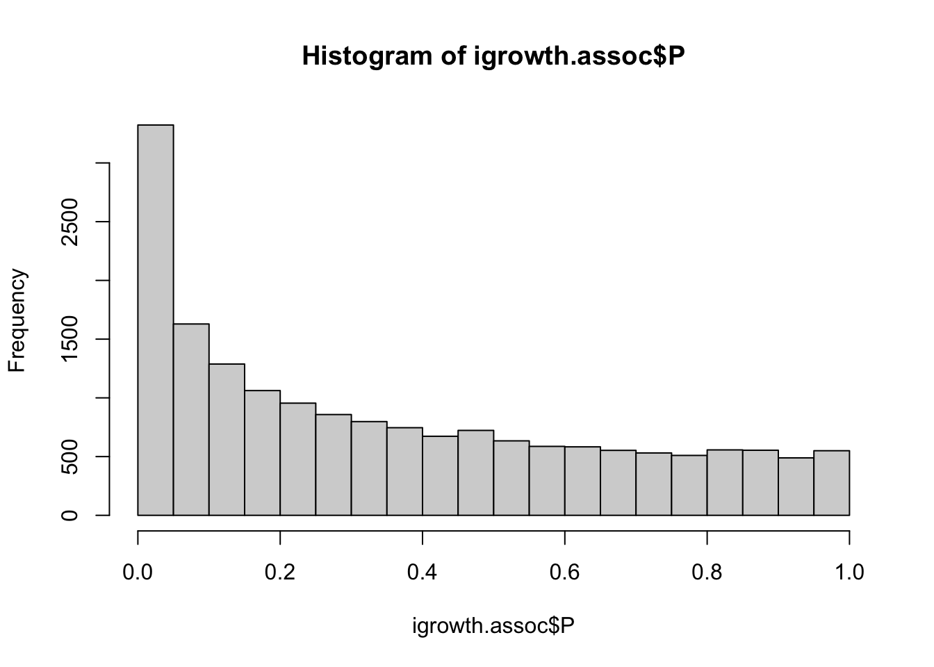

qqunif(igrowth.assoc$P)

## install.packages("qqman")
library(qqman)

##

## For example usage please run: vignette('qqman')

##

## Citation appreciated but not required:

## Turner, S.D. qqman: an R package for visualizing GWAS results using Q-Q and manhattan plots. biorXiv DOI: 10.1101/005165 (2014).

##

manhattan(igrowth.assoc, chr="CHR", bp="BP", snp="SNP", p="P" )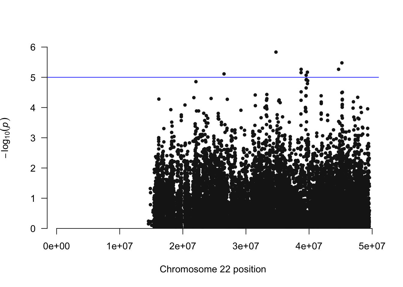

Calculate principal components using plink

## generate PCs using plink
if(!file.exists(glue::glue("{work.dir}output/pca.eigenvec")))
system(glue::glue("~/bin/plink --bfile {work.dir}hapmapch22 --pca --out {work.dir}output/pca"))
## read plink calculated PCs
pcplink = read.table(glue::glue("{work.dir}output/pca.eigenvec"),header=F, as.is=T)
names(pcplink) = c("FID","IID",paste0("PC", c(1:(ncol(pcplink)-2))) )
pcplink = popinfo %>% left_join(superpop,by=c("population"="Population")) %>% inner_join(pcplink, by=c("FID"="FID", "IID"="IID"))
## plot PC1 vs PC2
pcplink %>% ggplot(aes(PC1,PC2,col=population,shape=SuperPop)) + geom_point(size=3,alpha=.7) + theme_bw(base_size = 15)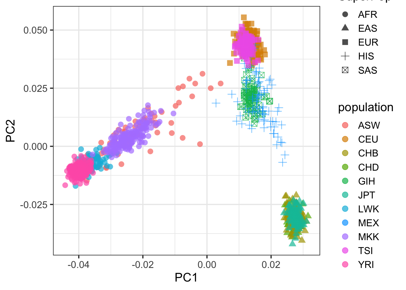

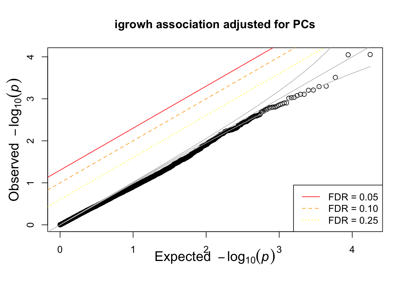
runnig igrowth GWAS using PCs

if(!file.exists(glue::glue("{work.dir}output/igrowth-adjPC.assoc.linear")))
system(glue::glue("~/bin/plink --bfile {work.dir}hapmapch22 --linear --pheno {work.dir}igrowth.pheno --pheno-name growth --covar {work.dir}output/pca.eigenvec --covar-number 1-4 --hide-covar --maf 0.05 --out {work.dir}output/igrowth-adjPC"))
igrowth.adjusted.assoc = read.table(glue::glue("{work.dir}output/igrowth-adjPC.assoc.linear"),header=T,as.is=T)
##indadd = igrowth.adjusted.assoc$TEST=="ADD"
titulo = "igrowh association adjusted for PCs"
hist(igrowth.adjusted.assoc$P,main=titulo)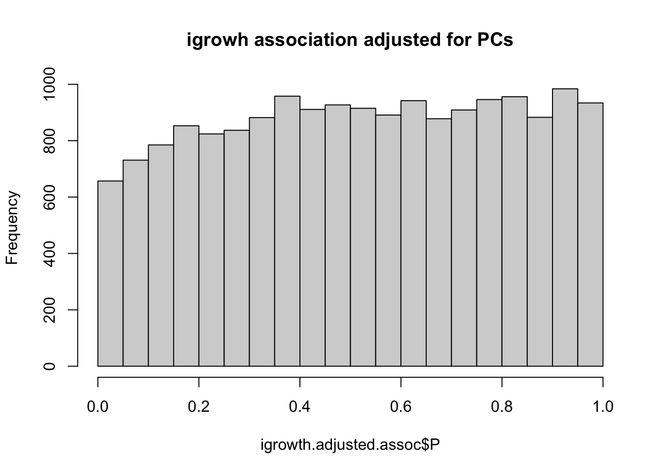

qqunif(igrowth.adjusted.assoc$P,main=titulo)