Multiple Testing

Learning objectives

• build intuition about p-values when multiple testing is performed via simulations
• recognize the need for multiple testing correction
• present methods to correct for multiple testing
  • Bonferroni correction
  • FDR (false discovery rate)

Motivate the need for multiple testing correction

## simulate two independent, normally distributed random variables X and epsi

## set seed to make simulations reproducible
set.seed(20210108)

## parameter definition
nsamp = 100
beta = 2
h2 = 0.1
sig2X = h2
sig2epsi = (1 - sig2X) * beta^2
sigX = sqrt(sig2X)
sigepsi = sqrt(sig2epsi)

## simulate normally distributed X and epsi
X = rnorm(nsamp,mean=0, sd= sigX)
epsi = rnorm(nsamp,mean=0, sd=sigepsi)

## let's look at the distribution of X and epsi
par(mfrow=c(2,1)) ## stacks two plots 
maxrango=range(c(X,epsi))
hist(X,xlim=maxrango)
hist(epsi,xlim=maxrango)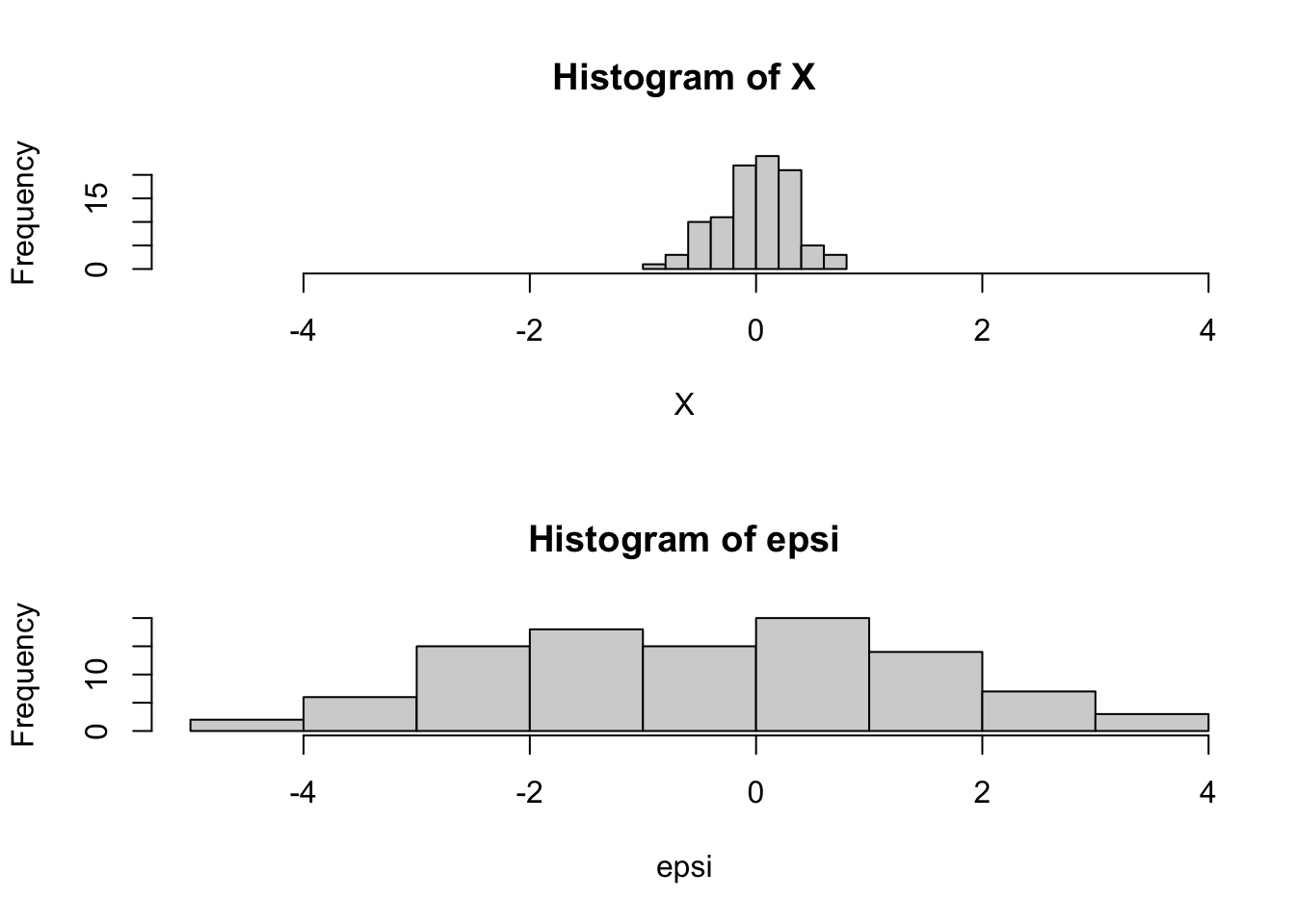

par(mfrow=c(1,1)) ## back to one plot format

## generate Yalt (X has an effect on Yalt)
Yalt = X * beta + epsi

## plot Yalt vs X
plot(X, Yalt, main="Yalt vs X")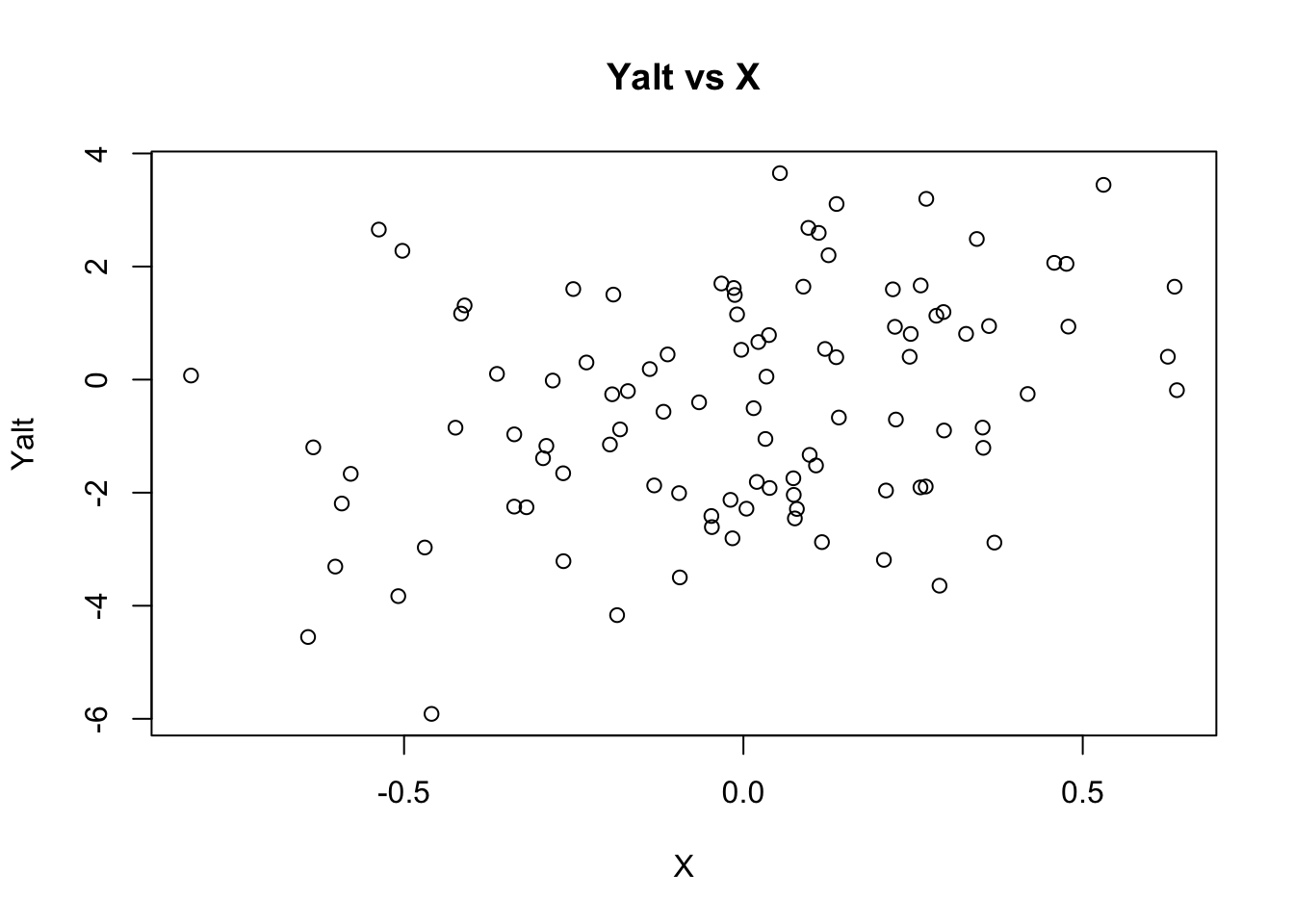

## generate Ynull (X has no effect on Ynull)
Ynull = rnorm(nsamp, mean=0, sd=beta)

## plot Ynull vs X
plot(X, Ynull, main="Ynull vs X")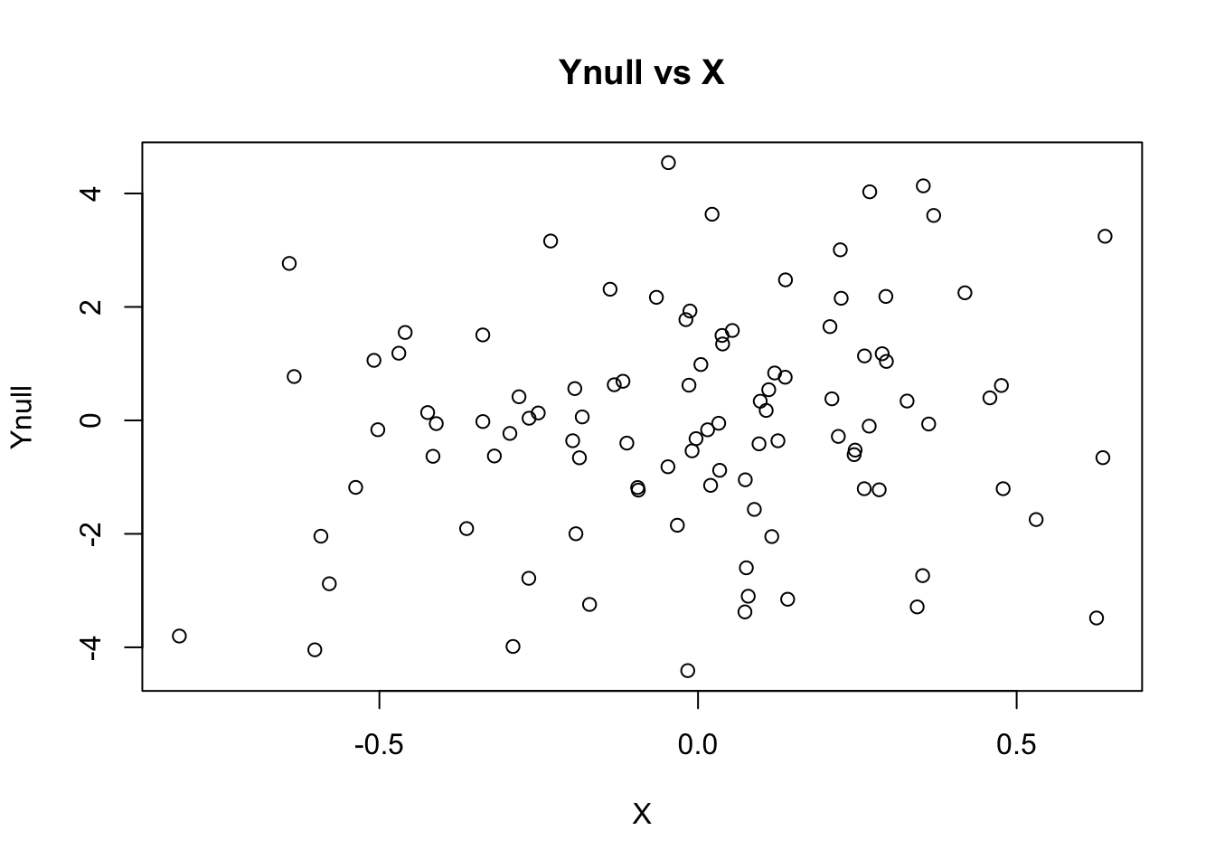

## let's compare the distributions of Ynull and Yalt

par(mfrow=c(2,1)) ## stacks two plots 
maxrango=range(c(Yalt,Ynull))
hist(Ynull,xlim=maxrango)
hist(Yalt,xlim=maxrango)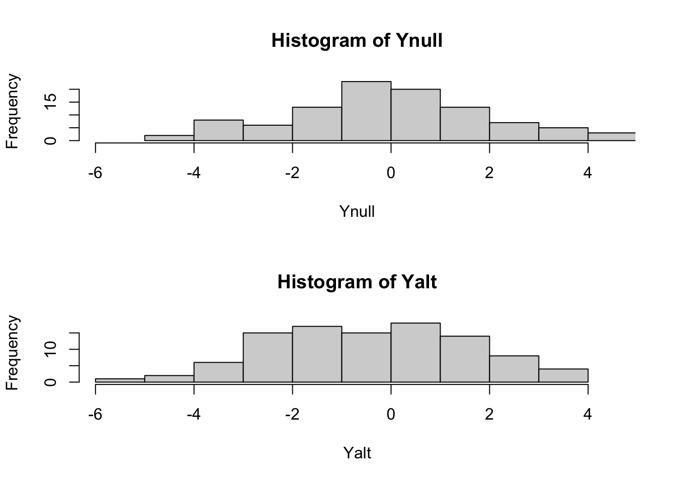

par(mfrow=c(1,1)) ## back to one plot format

## let's look at the qqplot of Yalt compared to the expected distribution for a normally distributed random variable
qqnorm(Yalt, main = paste("mean(Y) = ",signif(mean(Yalt),2),"; sd(Y) = ",signif(sd(Yalt),3))); qqline(Yalt)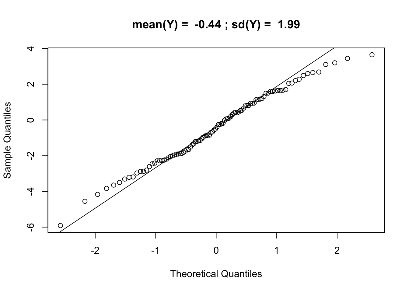

## let's look at the qqplot of Yalt compared to the expected distribution for a normally distributed random variable
qqplot(Ynull, Yalt, main="comparing Ynull and Yalt marginal distributions"); abline(0,1)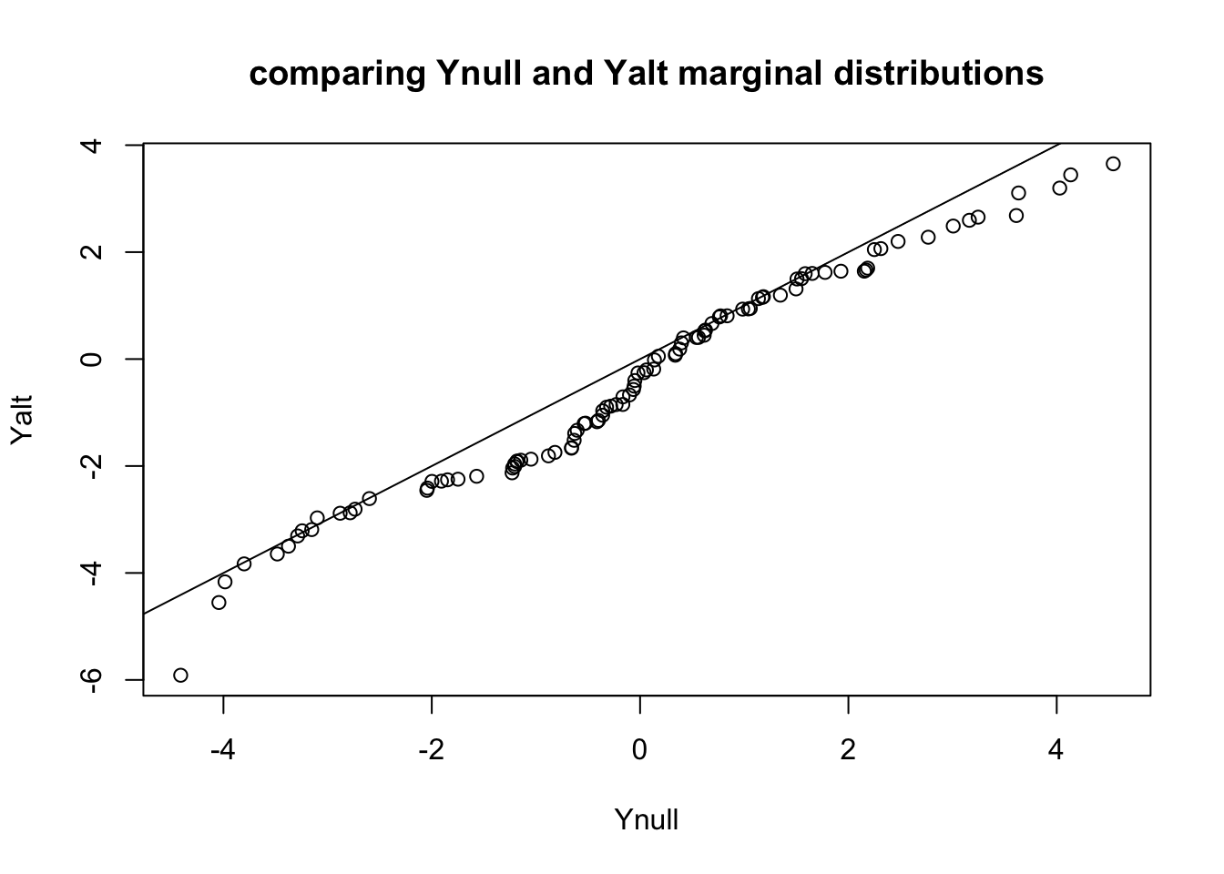

## let's formally test whether Ynull and Yalt are normally distributed
shapiro.test(Ynull)

## 
##  Shapiro-Wilk normality test
## 
## data:  Ynull
## W = 0.98746, p-value = 0.4692

shapiro.test(Yalt)

## 
##  Shapiro-Wilk normality test
## 
## data:  Yalt
## W = 0.98874, p-value = 0.5646

## test association between Ynull and X
summary(lm(Ynull ~ X))

## 
## Call:
## lm(formula = Ynull ~ X)
## 
## Residuals:
##     Min      1Q  Median      3Q     Max 
## -4.3548 -1.1589  0.0782  1.3735  4.6291 
## 
## Coefficients:
##             Estimate Std. Error t value Pr(>|t|)
## (Intercept)  -0.0395     0.1951  -0.202    0.840
## X             1.0095     0.6240   1.618    0.109
## 
## Residual standard error: 1.95 on 98 degrees of freedom
## Multiple R-squared:  0.02601,    Adjusted R-squared:  0.01607 
## F-statistic: 2.617 on 1 and 98 DF,  p-value: 0.1089

## what's the p-value of the association?

## is the p-value significant at 5% significance leve?

## what about Yalt and X?

summary(lm(Yalt ~ X))

## 
## Call:
## lm(formula = Yalt ~ X)
## 
## Residuals:
##     Min      1Q  Median      3Q     Max 
## -4.5453 -1.4809  0.1231  1.2189  4.1808 
## 
## Coefficients:
##             Estimate Std. Error t value Pr(>|t|)   
## (Intercept)  -0.4244     0.1891  -2.244   0.0271 * 
## X             2.0521     0.6050   3.392   0.0010 **
## ---
## Signif. codes:  0 '***' 0.001 '**' 0.01 '*' 0.05 '.' 0.1 ' ' 1
## 
## Residual standard error: 1.89 on 98 degrees of freedom
## Multiple R-squared:  0.1051, Adjusted R-squared:  0.09595 
## F-statistic: 11.51 on 1 and 98 DF,  p-value: 0.001001

## what's the p-value of the association?

## is the p-value significant at 5% significance level?

We want to run 10000 times this same regression, so here we define a function fastlm that will get us the p-values and regression coefficients.

fastlm = function(xx,yy)
{
  ## compute betahat (regression coef) and pvalue with Ftest
  ## for now it does not take covariates
  
  df1 = 2
  df0 = 1
  ind = !is.na(xx) & !is.na(yy)
  xx = xx[ind]
  yy = yy[ind]
  n = sum(ind)
  xbar = mean(xx)
  ybar = mean(yy)
  xx = xx - xbar
  yy = yy - ybar
  
  SXX = sum( xx^2 )
  SYY = sum( yy^2 )
  SXY = sum( xx * yy )
  
  betahat = SXY / SXX
  
  RSS1 = sum( ( yy - xx * betahat )^2 )
  RSS0 = SYY
  
  fstat = ( ( RSS0 - RSS1 ) / ( df1 - df0 ) )  / ( RSS1 / ( n - df1 ) )
  pval = 1 - pf(fstat, df1 = ( df1 - df0 ), df2 = ( n - df1 ))
  res = list(betahat = betahat, pval = pval)
  
  return(res)
}

Simulate distribution of p-values under the null

## load some useful functions such as fastlm, a fast enough function to run regression ten thousand of times within a reasonable time

## source("myfunctions.r")

nsim = 10000
# ## parameter definition
# use definition above
# nsamp = 100
# beta = 2
# h2 = 0.3
# sig2X = h2
# sig2epsi = (1 - sig2X) * beta^2
# sigX = sqrt(sig2X)
# sigepsi = sqrt(sig2epsi)

## simulate normally distributed X and epsi
Xmat = matrix(rnorm(nsim * nsamp,mean=0, sd= sigX), nsamp, nsim)
epsimat = matrix(rnorm(nsim * nsamp,mean=0, sd=sigepsi), nsamp, nsim)

## generate Yalt (X has an effect on Yalt)
Ymat_alt = Xmat * beta + epsimat

## generate Ynull (X has no effect on Ynull)
Ymat_null = matrix(rnorm(nsim * nsamp, mean=0, sd=beta), nsamp, nsim)

## let's look at the dimensions of the simulated matrices

dim(Ymat_null)

## [1]   100 10000

dim(Ymat_alt)

## [1]   100 10000

## Now we have 10000 independent simulations of X, Ynull, and Yalt

## give them names so that we can refer to them later more easily

colnames(Ymat_null) = paste0("c",1:ncol(Ymat_null))
colnames(Ymat_alt) = colnames(Ymat_null)

## Let's run 10000 linear regressions of the time Ynull = X*b + epsilon, to do this in a reasonable amount of time, we will use the fastlm function we loaded 

pvec = rep(NA,nsim)
bvec = rep(NA,nsim)

for(ss in 1:nsim)
{
  fit = fastlm(Xmat[,ss], Ymat_null[,ss])
  pvec[ss] = fit$pval  
  bvec[ss] = fit$betahat
}

summary(pvec)

##      Min.   1st Qu.    Median      Mean   3rd Qu.      Max. 
## 0.0000021 0.2438476 0.4903663 0.4935828 0.7401156 0.9998408

hist(pvec,xlab="p-value",main="Histogram of p-values under Null")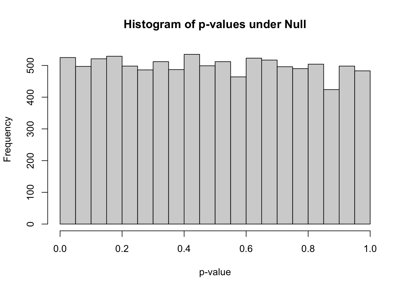

• how many simulations under the null yield p-value below 0.05? What percentage is that?

sum(pvec<0.05)

## [1] 525

mean(pvec<0.05)

## [1] 0.0525

• how many simulations under the null yield p-value < 0.20?

• Why do we need to use more stringent significance level when we test many times?

Bonferroni correction

Use as the new threshold the original one divided by the number of tests. So typically

\[\frac{0.05}{\text{total number of tests}}\]

• what’s the Bonferroni threshold for significance in this simulation?

• how many did we find?

BF_thres = 0.05/nsim
## Bonferroni significance threshold
print(BF_thres) 

## [1] 5e-06

## number of Bonferroni significant associations
sum(pvec<BF_thres)

## [1] 1

## proportion of Bonferroni significant associations
mean(pvec<BF_thres)

## [1] 1e-04

GWAS significance threshold

The consensus value for calling a GWAS hit significant it \(5\cdot 10^{-8}\). How many tests are we correcting the usual 0.05 threshold?

Current GWAS have typically 10 million SNPs but we still use \(5\cdot 10^{-8}\). What do you think is the justification?

Mix of Ynull and Yalt

Let’s see what happens when we add a bunch of true associations in the matrix of null associations

prop_alt=0.20 ## define proportion of alternative Ys in the mixture
selectvec = rbinom(nsim,1,prop_alt)
names(selectvec) = colnames(Ymat_alt)
selectvec[1:10]

##  c1  c2  c3  c4  c5  c6  c7  c8  c9 c10 
##   1   0   0   0   1   1   0   0   0   1

Ymat_mix = sweep(Ymat_alt,2,selectvec,FUN='*') + sweep(Ymat_null,2,1-selectvec,FUN='*')
## Ymat_mix should have Yalt for columns that have 1's in selectvec and Ynull where selectvec==0
print(head(Ymat_mix[,1:10]),2) ## use 2 decimals

##         c1   c2    c3    c4      c5     c6     c7     c8    c9   c10
## [1,]  1.72 -0.4 -1.06  2.49  0.6637 -0.021 -0.024  4.177 -2.39  2.46
## [2,]  0.72 -2.1 -0.64  0.30  1.7522 -1.704  1.457 -0.085 -1.67  0.33
## [3,] -1.58  1.4  2.55  0.65 -2.0064 -0.427  3.817 -2.514 -1.54  1.90
## [4,]  1.06  1.1 -1.99  0.32  2.0433  0.792  0.255 -0.567 -1.43  0.06
## [5,] -1.55 -3.9 -0.53  1.45 -0.0054  1.736 -0.681  1.339 -0.68 -0.55
## [6,]  2.71  1.6 -0.83 -1.70 -1.1723  0.882 -1.150  4.442 -2.68 -3.95

print(selectvec[1:10])

##  c1  c2  c3  c4  c5  c6  c7  c8  c9 c10 
##   1   0   0   0   1   1   0   0   0   1

print("subtract Ymat_alt")

## [1] "subtract Ymat_alt"

print(head(Ymat_mix[,1:10] - Ymat_alt[,1:10]),2)

##      c1    c2     c3     c4 c5 c6   c7    c8    c9 c10
## [1,]  0 -1.33 -0.094  3.130  0  0  2.0  2.46 -0.96   0
## [2,]  0 -2.59  3.562  1.311  0  0  1.4  4.67 -1.76   0
## [3,]  0  1.05  0.273 -0.045  0  0  4.4 -3.20  3.70   0
## [4,]  0  3.29 -0.959  5.577  0  0 -1.8 -0.22 -0.71   0
## [5,]  0 -3.81 -1.331  3.413  0  0 -3.4  0.55 -4.43   0
## [6,]  0 -0.73 -0.381 -3.416  0  0 -1.7  5.82 -3.14   0

print("subtract Ymat_null")

## [1] "subtract Ymat_null"

print(head(Ymat_mix[,1:10] - Ymat_null[,1:10]),2)

##         c1 c2 c3 c4    c5    c6 c7 c8 c9   c10
## [1,]  2.91  0  0  0  1.62 -0.69  0  0  0  0.47
## [2,] -1.41  0  0  0  2.63  0.20  0  0  0  3.51
## [3,] -2.19  0  0  0 -0.99  1.64  0  0  0  2.77
## [4,]  0.57  0  0  0  5.23  3.09  0  0  0 -0.50
## [5,] -4.57  0  0  0 -0.68 -1.97  0  0  0  2.19
## [6,]  3.57  0  0  0 -4.26  2.85  0  0  0 -4.06

## Q: how many columns have true effect and how many have null effects
sum(selectvec)

## [1] 2004

mean(selectvec)

## [1] 0.2004

## run linear regression for all 10000 phenotypes in the mix of true and false associations, Ymat_mix
pvec_mix = rep(NA,nsim)
bvec_mix = rep(NA,nsim)
for(ss in 1:nsim)
{
  fit = fastlm(Xmat[,ss], Ymat_mix[,ss])
  pvec_mix[ss] = fit$pval  
  bvec_mix[ss] = fit$betahat
}
summary(pvec_mix)

##    Min. 1st Qu.  Median    Mean 3rd Qu.    Max. 
## 0.00000 0.07854 0.37313 0.40036 0.67907 0.99984

hist(pvec_mix,xlab="p-value",main="Histogram of p-values under Null")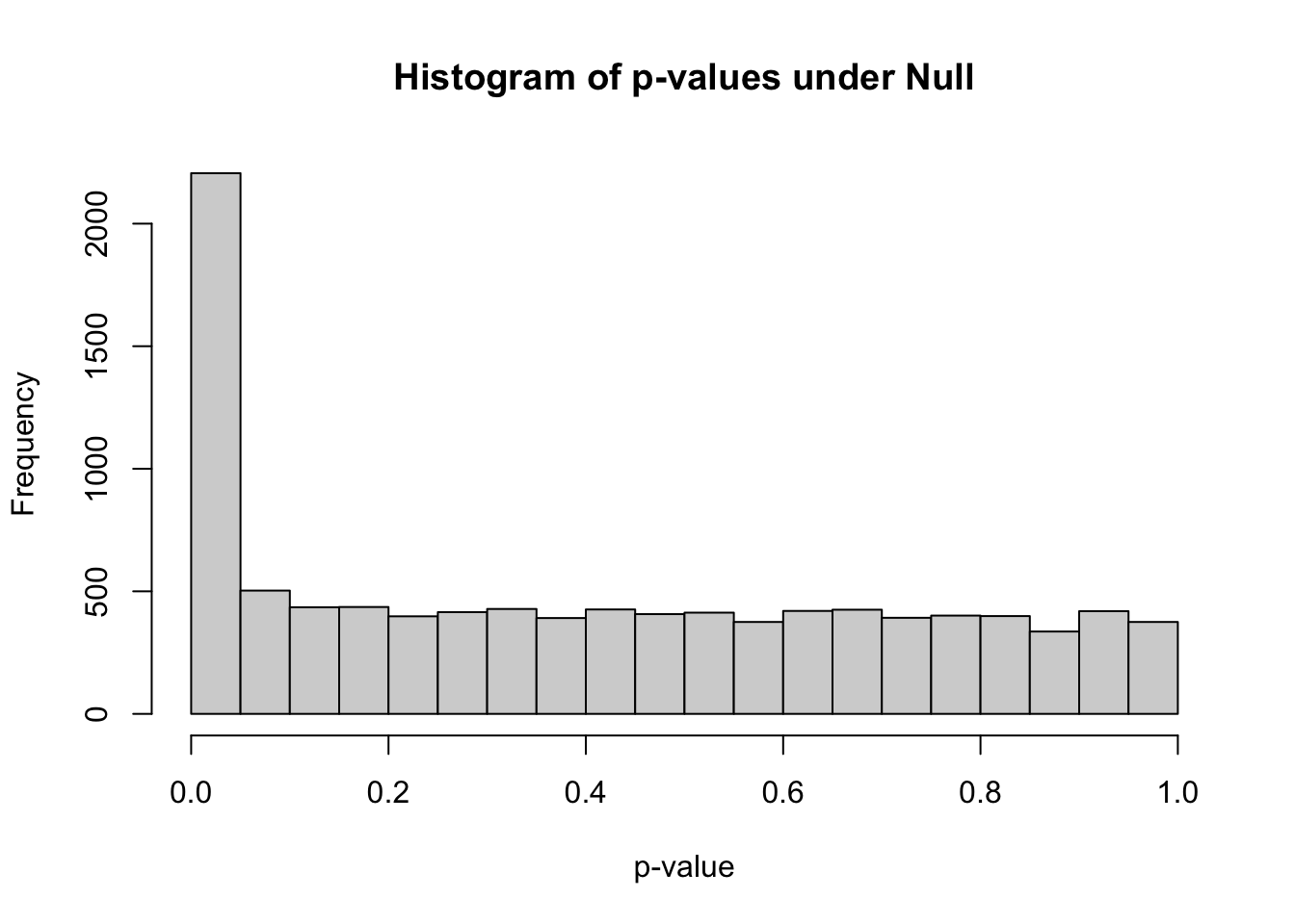

m_signif = sum(pvec_mix < 0.05) ## observed number of significant associations
m_expected = 0.05*nsim ## expected number of significant associations under the worst case scenario, where all features belong to the null 
m_signif

## [1] 2206

m_expected

## [1] 500

Under the null, we were expecting 500 significant columns by chance but got 2206

Q: how can we estimate the proportion of true positives?

We got 1706 extra columns, so it’s reasonable to expect that the extra significant results come from the alternative distribution (Yalt). So \[\frac{\text{observed number of significant} - \text{expected number of significant}}{\text{observed number of significant}}\] should be a good estimate of the true discovery rate. False discovery rate is defined as 1 - the true discovery rate.

Fortunately, since we simulated this data, we know the number of true associations.

## loading my qqunif function
devtools::source_gist("https://gist.github.com/hakyim/38431b74c6c0bf90c12f")

## Sourcing https://gist.githubusercontent.com/hakyim/38431b74c6c0bf90c12f/raw/fe087cf0519d4a3d71f0c8235f42cce4549438ac/qqunif.R

## SHA-1 hash of file is 0b30870726d50889d1366a1f3b21942510a05128

qqunif(pvec)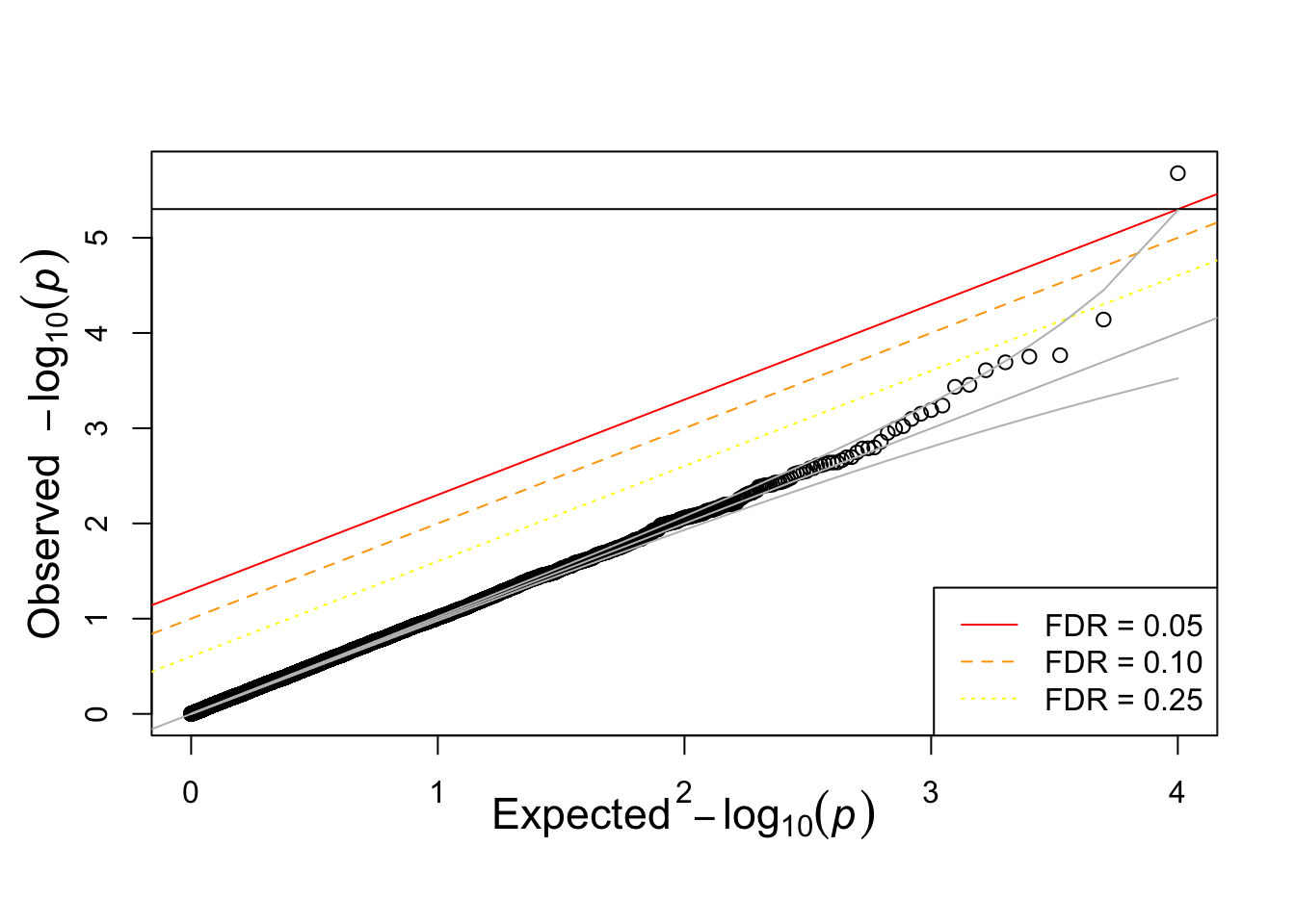

qqunif(pvec_mix)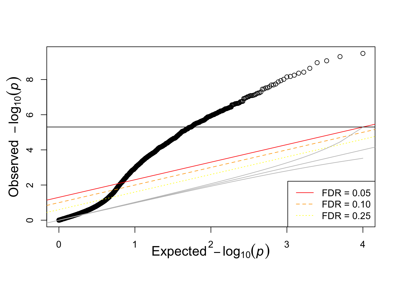

ind=order(pvec_mix,decreasing=FALSE)
qqunif(pvec_mix,col=selectvec[ind]+1)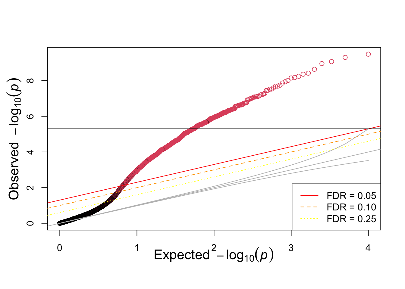

table(pvec_mix<0.05, selectvec)

##        selectvec
##            0    1
##   FALSE 7580  214
##   TRUE   416 1790

count_table = t(table(pvec_mix>0.05, selectvec))
colnames(count_table) = c("Called significant", "Called not significant")
rownames(count_table) = c("Null true", "Alt true")
knitr::kable(count_table)

	Called significant	Called not significant
Null true	416	7580
Alt true	1790	214

Common approaches to control type I errors

Assuming we are testing \(m\) hypothesis, let’s the following terms for the different errors.

	Called Significant	Called not significant	Total
Null true	\(F\)	\(m_0 - F\)	\(m_0\)
Alt true	\(T\)	\(m_1 - T\)	\(m_1\)
Total	\(S\)	\(m - S\)	\(m\)

• Bonferroni correction assures that the FWER (Familywise error rate) \[P(F \ge 1)\] is below the acceptable type I error, typically 0.05. This can be too stringent and lead to miss real signals.
• pFDR (positive false discovery rate) \[E\left(\frac{F}{S} \rvert S>0\right)\]
• qvalue is the minimum false discovery rate attainable when the feature (SNP) is called significant

Let’s calculate the qvalue

Use qvalue package to calculate FDR and

if (!requireNamespace("BiocManager", quietly = TRUE))
    install.packages("BiocManager")

BiocManager::install("qvalue")

Let’s check whether small qvalues correspond to true associations (i.e. the phenotype was generated under the alternative distribution)

qres_mix = qvalue::qvalue(pvec_mix)
qvec_mix = qres_mix$qvalue

plot(qvec_mix,col=selectvec*2 + 1, pch=selectvec + 1, lwd=selectvec*2 + 1)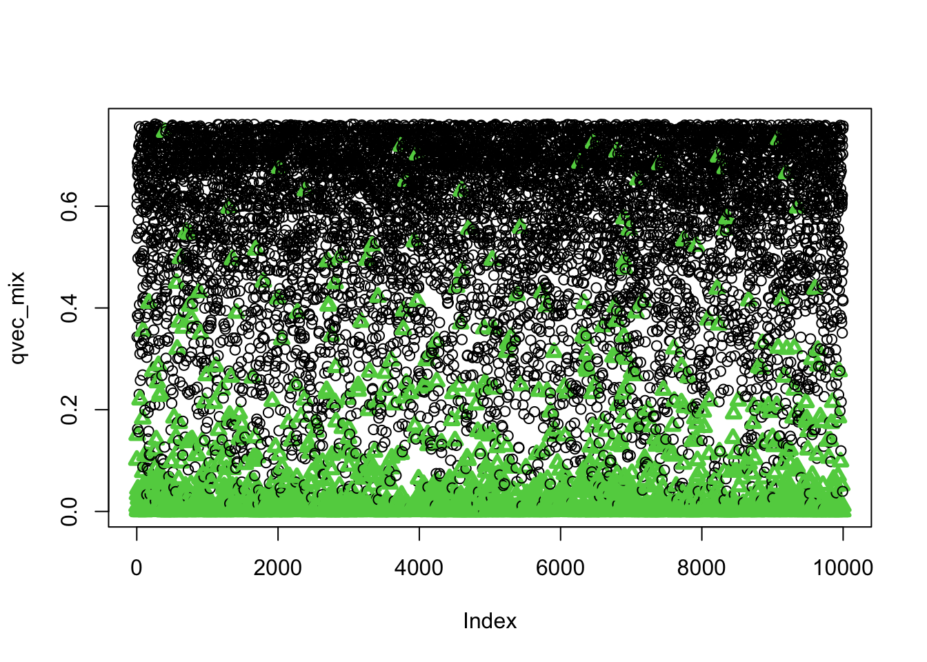 

## using selectvec*2 + 1 as a quick way to get the vector to be 1 and 3 (1 is black 3 is green) instead of 1 and 2 (2 is read and can be difficult to read for color blind people)

ind=order(qvec_mix,decreasing=FALSE)
plot(sort(qvec_mix),col=selectvec[ind]*2 + 1, pch=selectvec[ind] + 1, lwd=selectvec[ind]*2 + 1)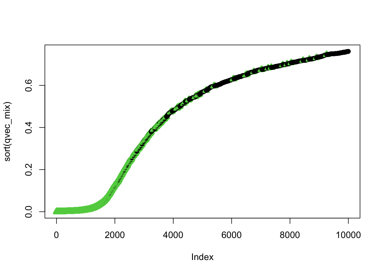 

summary(qvec_mix)

##      Min.   1st Qu.    Median      Mean   3rd Qu.      Max. 
## 0.0000019 0.2391430 0.5681539 0.4635186 0.6894836 0.7615203