Lecture 3 Association I

Haky Im

2021-01-19

Categories: Lecture

Learning Objectives

Differentiate Mendelian vs. Complex Disease
Compare linkage vs association methods
Review hypothesis testing
Review regression approaches
Explain GWAS
Read the WTCCC 2007 GWAS study
Interpret Manhattan and QQ plots
Recognize the need for multiple testing correction
- p-values under the null distribution
- Bonferroni correction
- False positive rates

Material for the class

Download notes from here
Claussnitzer et al. (2020). A brief history of human disease genetics. http://doi.org/10.1038/s41586-019-1879-7
Notes on multiple testing here

Monogenic/Mendelian vs Complex traits

Methods for gene mapping

Hypothesis testing

Regression with single SNP

GWAS

Welcome Trust example

Multiple testing correction

See the full vignette here

## simulate two independent, normally distributed random variables X and epsi

## set seed to make simulations reproducible
set.seed(20210108)

## parameter definition
nsamp = 100
beta = 2
h2 = 0.6
sig2X = h2
sig2epsi = (1 - sig2X) * beta^2
sigX = sqrt(sig2X)
sigepsi = sqrt(sig2epsi)

## simulate normally distributed X and epsi
X = rnorm(nsamp,mean=0, sd= sigX)
epsi = rnorm(nsamp,mean=0, sd=sigepsi)

## let's look at the distribution of X and epsi
par(mfrow=c(2,1)) ## stacks two plots 
maxrango=range(c(X,epsi))
hist(X,xlim=maxrango)
hist(epsi,xlim=maxrango)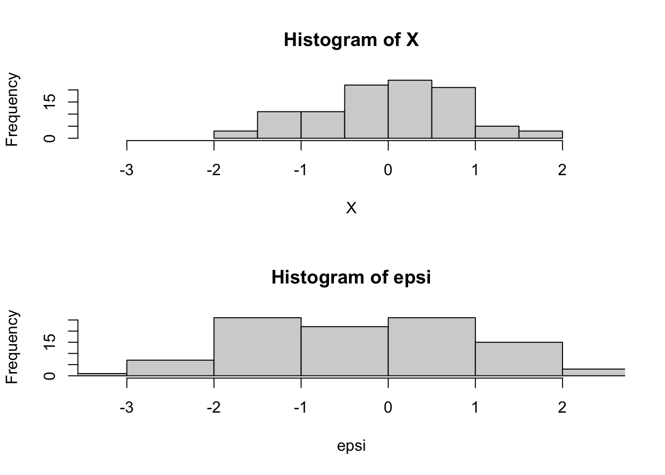

par(mfrow=c(1,1)) ## back to one plot format

## generate Yalt (X has an effect on Yalt)
Yalt = X * beta + epsi

## plot Yalt vs X
plot(X, Yalt, main="Yalt vs X")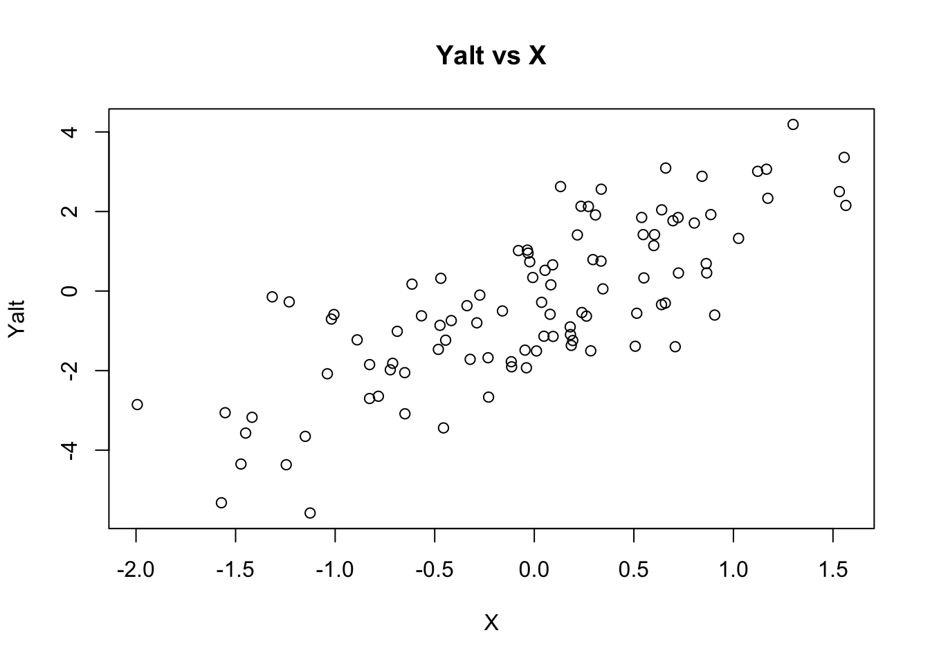

## generate Ynull (X has no effect on Ynull)
Ynull = rnorm(nsamp, mean=0, sd=beta)

## plot Ynull vs X
plot(X, Ynull, main="Ynull vs X")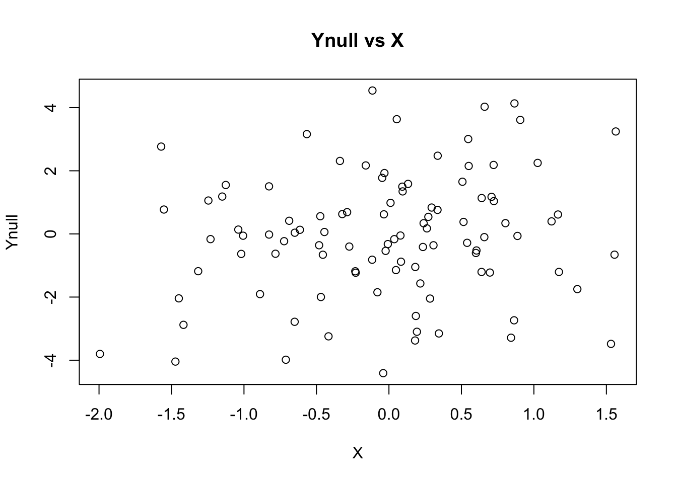

## let's compare the distributions of Ynull and Yalt

par(mfrow=c(2,1)) ## stacks two plots 
maxrango=range(c(Yalt,Ynull))
hist(Ynull,xlim=maxrango)
hist(Yalt,xlim=maxrango)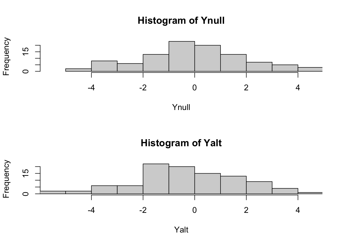

par(mfrow=c(1,1)) ## back to one plot format



## let's look at the qqplot of Yalt compared to the expected distribution for a normally distributed random variable
qqnorm(Yalt, main = paste("mean(Y) = ",signif(mean(Yalt),2),"; sd(Y) = ",signif(sd(Yalt),3))); qqline(Yalt)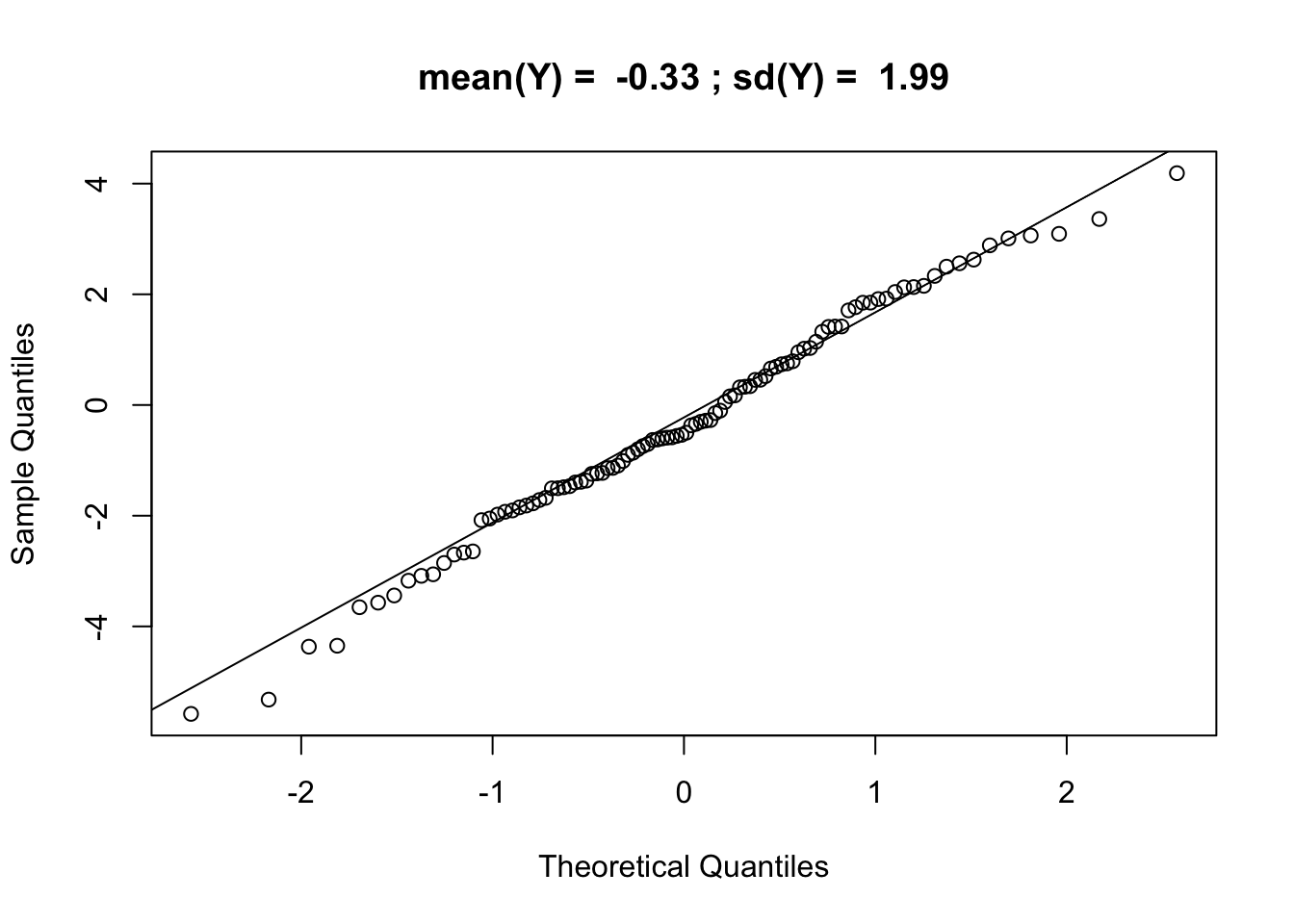

## let's look at the qqplot of Yalt compared to the expected distribution for a normally distributed random variable
qqplot(Ynull, Yalt, main="comparing Ynull and Yalt marginal distributions"); abline(0,1)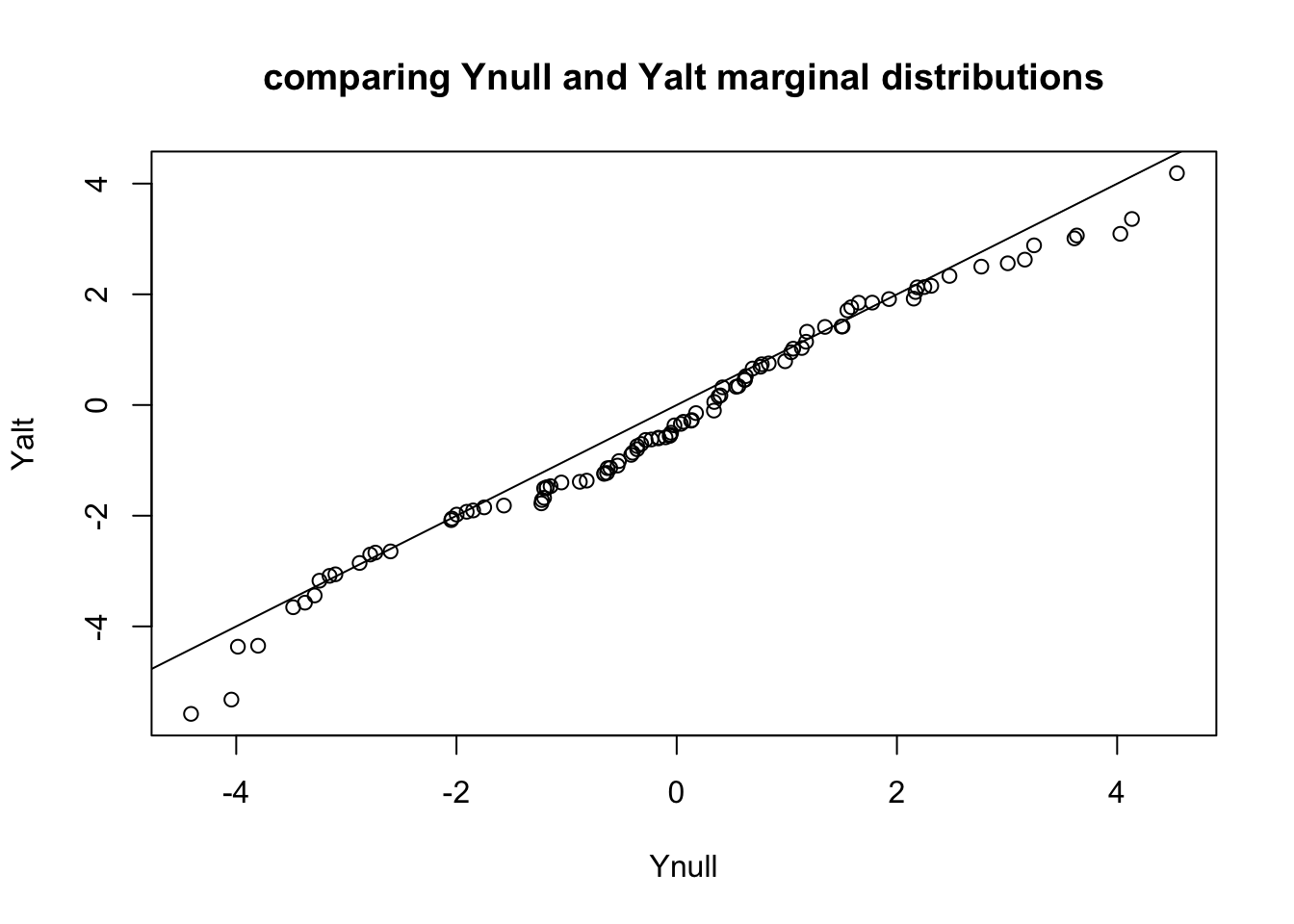

## let's formally test whether Ynull and Yalt are normally distributed
shapiro.test(Ynull)

## 
##  Shapiro-Wilk normality test
## 
## data:  Ynull
## W = 0.98746, p-value = 0.4692

shapiro.test(Yalt)

## 
##  Shapiro-Wilk normality test
## 
## data:  Yalt
## W = 0.99031, p-value = 0.69

## test association between Ynull and X

summary(lm(Ynull ~ X))

## 
## Call:
## lm(formula = Ynull ~ X)
## 
## Residuals:
##     Min      1Q  Median      3Q     Max 
## -4.3548 -1.1589  0.0782  1.3735  4.6291 
## 
## Coefficients:
##             Estimate Std. Error t value Pr(>|t|)
## (Intercept)  -0.0395     0.1951  -0.202    0.840
## X             0.4122     0.2548   1.618    0.109
## 
## Residual standard error: 1.95 on 98 degrees of freedom
## Multiple R-squared:  0.02601,    Adjusted R-squared:  0.01607 
## F-statistic: 2.617 on 1 and 98 DF,  p-value: 0.1089

## what's the p-value of the association?

## is the p-value significant at 5% significance leve?

## what about Yalt and X?

summary(lm(Yalt ~ X))

## 
## Call:
## lm(formula = Yalt ~ X)
## 
## Residuals:
##     Min      1Q  Median      3Q     Max 
## -3.0302 -0.9873  0.0821  0.8126  2.7872 
## 
## Coefficients:
##             Estimate Std. Error t value Pr(>|t|)    
## (Intercept)  -0.2829     0.1261  -2.244   0.0271 *  
## X             2.0142     0.1646  12.233   <2e-16 ***
## ---
## Signif. codes:  0 '***' 0.001 '**' 0.01 '*' 0.05 '.' 0.1 ' ' 1
## 
## Residual standard error: 1.26 on 98 degrees of freedom
## Multiple R-squared:  0.6043, Adjusted R-squared:  0.6002 
## F-statistic: 149.7 on 1 and 98 DF,  p-value: < 2.2e-16

## what's the p-value of the association?

## is the p-value significant at 5% significance level?

Simulate distribution of p-values under the null

## load some useful functions such as fastlm, a fast enough function to run regression ten thousand of times within a reasonable time

source("myfunctions.r")

nsim = 10000
## parameter definition
nsamp = 100
beta = 2
h2 = 0.6
sig2X = h2
sig2epsi = (1 - sig2X) * beta^2
sigX = sqrt(sig2X)
sigepsi = sqrt(sig2epsi)

## simulate normally distributed X and epsi
Xmat = matrix(rnorm(nsim * nsamp,mean=0, sd= sigX), nsamp, nsim)
epsimat = matrix(rnorm(nsim * nsamp,mean=0, sd=sigepsi), nsamp, nsim)

## generate Yalt (X has an effect on Yalt)
Ymat_alt = Xmat * beta + epsimat

## generate Ynull (X has no effect on Ynull)
Ymat_null = matrix(rnorm(nsim * nsamp, mean=0, sd=beta), nsamp, nsim)

## let's look at the dimensions of the simulated matrices

dim(Ymat_null)

## [1]   100 10000

dim(Ymat_alt)

## [1]   100 10000

## Now we have 10000 independent simulations of X, Ynull, and Yalt

## give them names so that we can refer to them later more easily

colnames(Ymat_null) = paste0("c",1:ncol(Ymat_null))
colnames(Ymat_alt) = colnames(Ymat_null)

## Let's run 10000 linear regressions of the time Ynull = X*b + epsilon, to do this in a reasonable amount of time, we will use the fastlm function we loaded 

pvec = rep(NA,nsim)
bvec = rep(NA,nsim)

for(ss in 1:nsim)
{
  fit = fastlm(Xmat[,ss], Ymat_null[,ss])
  pvec[ss] = fit$pval  
  bvec[ss] = fit$betahat
}

summary(pvec)

##      Min.   1st Qu.    Median      Mean   3rd Qu.      Max. 
## 0.0000021 0.2438476 0.4903663 0.4935828 0.7401156 0.9998408

hist(pvec,xlab="p-value",main="Histogram of p-values under Null")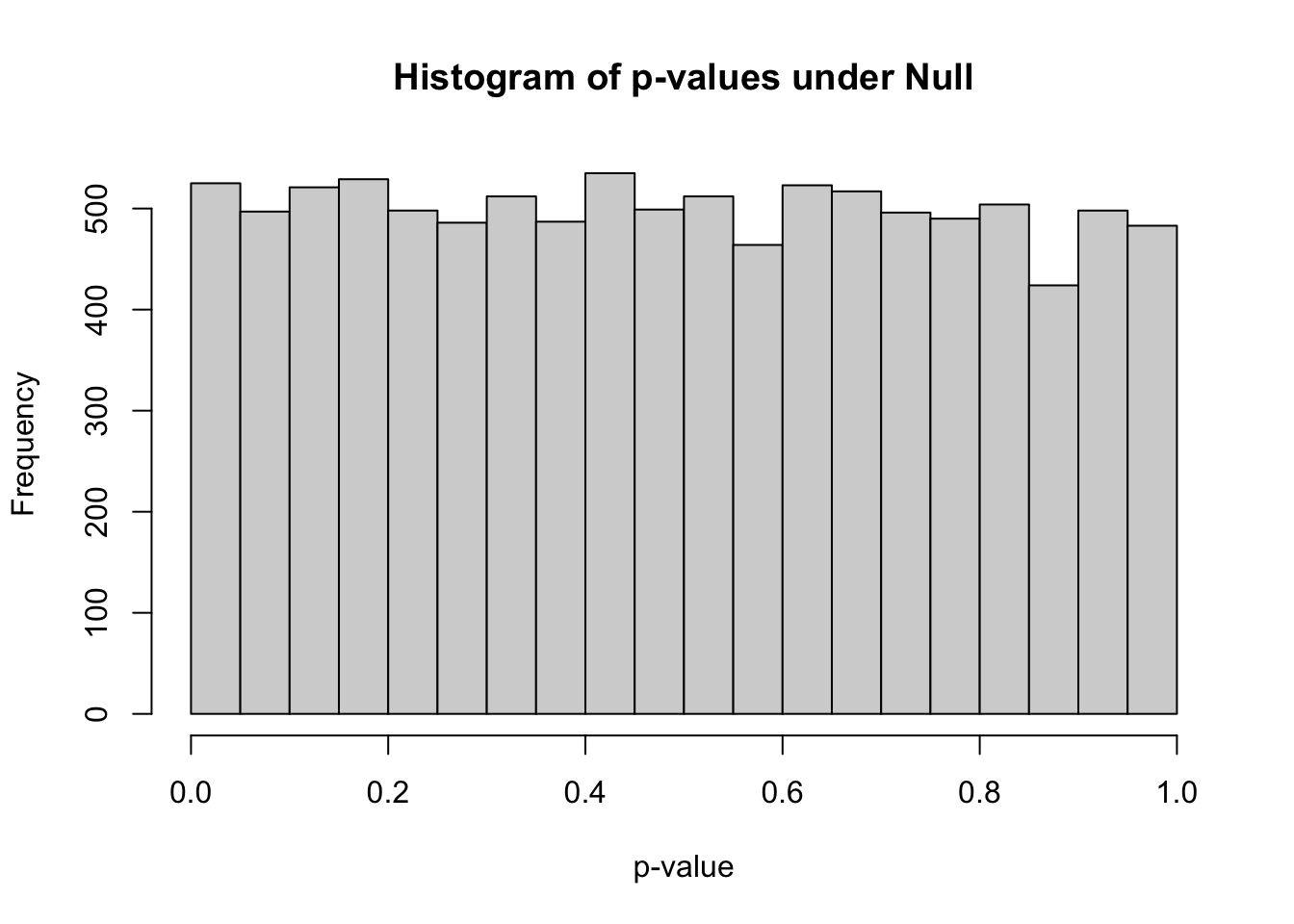

how many simulations under the null yield p-value below 0.05? What percentage is that?

sum(pvec<0.05)

## [1] 525

mean(pvec<0.05)

## [1] 0.0525

how many simulations under the null yield p-value < 0.20?
Why do we need to use more stringent significance level when we test many times?

Bonferroni correction

Use as the new threshold the original one divided by the number of tests. So typically

\[\frac{0.05}{\text{total number of tests}}\]

what’s the Bonferroni threshold for significance in this simulation?
how many did we find?

BF_thres = 0.05/nsim
## number of Bonferroni significant associations
sum(pvec<BF_thres)

## [1] 1

## proportion of Bonferroni significant associations
mean(pvec<BF_thres)

## [1] 1e-04

GWAS significance threshold

The consensus value for calling a GWAS hit significant it \(5\cdot 10^{-8}\). How many tests are we correcting the usual 0.05 threshold?

Current GWAS have typically 10 million SNPs but we still use \(5\cdot 10^{-8}\). What do you think is the justification?

Install qvalue package if you don’t already have it

if (!requireNamespace("BiocManager", quietly = TRUE))
    install.packages("BiocManager")

BiocManager::install("qvalue")

qres = qvalue::qvalue(pvec)
qvec = qres$qvalue
plot(sort(qvec))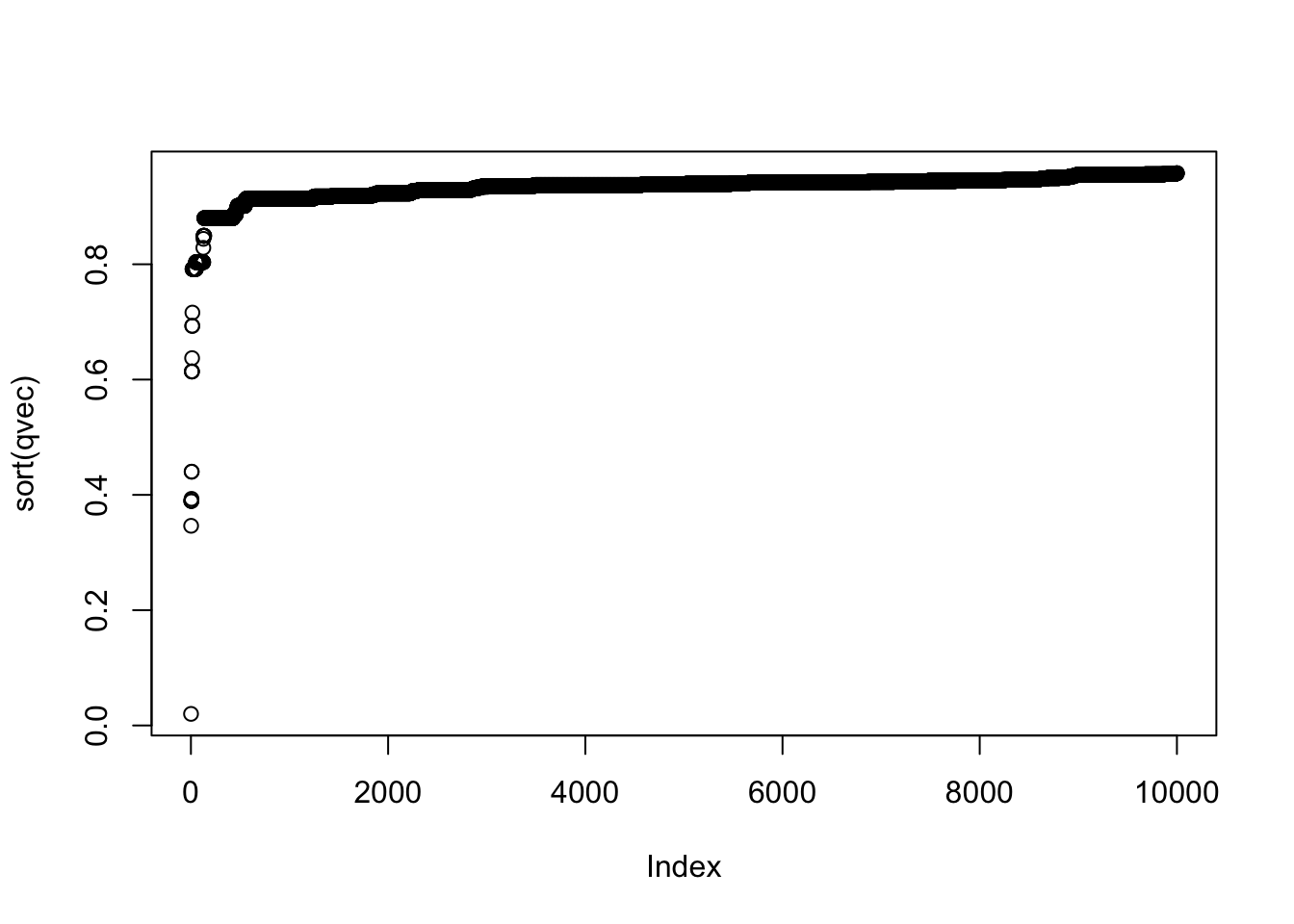

summary(qvec)

##    Min. 1st Qu.  Median    Mean 3rd Qu.    Max. 
##  0.0201  0.9288  0.9390  0.9333  0.9446  0.9580